Homework # 4 Solutions
Math 232, Spring 2012
Instructor: Dr. Doreen De Leon
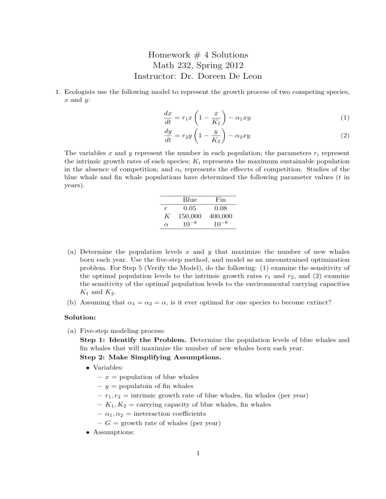
1. Ecologists use the following model to represent the growth process of two competing species, x and y : dx dt x
= r
1 x 1 −
K
1 dy dt y
= r
2 y 1 −
K
2
−
−
α
α
1
2 xy xy
(1)
(2)
The variables x and y represent the number in each population; the parameters r i represent the intrinsic growth rates of each species; K i in the absence of competition; and α i represents the maximum sustainable population represents the effeccts of competition. Studies of the blue whale and fin whale populations have determined the following parameter values ( t in years).
Blue Fin r 0.05
0.08
K 150,000 400,000
α 10
− 8 10
− 8
(a) Determine the population levels x and y that maximize the number of new whales born each year. Use the five-step method, and model as an unconstrained optimization problem. For Step 5 (Verify the Model), do the following: (1) examine the sensitivity of the optimal population levels to the intrinsic growth rates r
1 and r
2
, and (2) examine the sensitivity of the optimal population levels to the environmental carrying capacities
K
1 and K
2
.
(b) Assuming that α
1
= α
2
= α , is it ever optimal for one species to become extinct?
Solution:
(a) Five-step modeling process:
Step 1: Identify the Problem.
Determine the population levels of blue whales and fin whales that will maximize the number of new whales born each year.
Step 2: Make Simplifying Assumptions.
• Variables:
– x = population of blue whales
– y = populatoin of fin whales
– r
1
, r
2
= intrinsic growth rate of blue whales, fin whales (per year)
– K
1
, K
2
= carrying capacity of blue whales, fin whales
– α
1
, α
2
= ineteraction coefficients
– G = growth rate of whales (per year)
• Assumptions:
1

– The blue and fin whale populations may be modeled by the system in (1).
– r
1
= 0 .
05 , r
2
= 0 .
08
– K
1
= 150000 , K
2
= 400000
– α
1
= α
2 dx
– G = dt
– x, y ≥ 0
= 10
− 8
+ dy dt
Step 3: Construct the Model.
In this case, we wish to maximize the number of new whales born each year (i.e., to maximize the growth rate of the whales). From above, the growth rate of the whales is given by
G = dx
+ dt dy dt x
= r
1 x 1 −
K
1
− α
1 xy + r
2 y 1 − y
K
2
− α
2 xy
Therefore, substituting in the values for the parameters gives x
G ( x, y ) = 0 .
05 x 1 −
150000
+ 0 .
08 y 1 − y
400000
− 2 · 10
− 8 xy.
(3)
Our goal is to maximize G ( x, y ) over the set { ( x, y ) : x ≥ 0 , y ≥ 0 } .
Step 4: Solve and Interpret the Model.
Solving (see Maple worksheet) gives x ≈ 69104 , y ≈ 196545. At this point, the growth rate is G ( x, y ) ≈ 9589. So, the optimum population levels of blue and fin whales to maximize growth rate is 69,104 blue whales and 196,545 fin whales, resulting in a growth rate of 9.589 whales per year.
Step 5: Verify the Model.
We need to compute several sensitivities. The work for this is done in the Maple worksheet ( hw4sols.mw
).
i. Sensitivity of x and y with respect to r
1
.
G ( x, y, r
1
) = r
1
0 =
0 = x
∂G
∂x
∂G
∂y
1
=
− r
1 x
150000
−
2 r
1 x
150000
+ 0 .
08 y 1 −
− 2 · 10
− 8 y
= 0 .
08 − y
250000
− 2 · 10
− 8 x y
400000
Solving gives
− x = y =
120000000(250 r
1
− 1)
,
40000 r
1
− 3
7850000000 r
1
,
40000 r
1
− 3 both of which are valid for r
1
<
3
40000
. Then, the sensitivities are
S ( x, r
1
) =
S ( y, r
1
) = dx dr
1
· r
1 x ( r
1
)
≈ 0 .
085 r
1
=0 .
05 dy dr
1
· r
1 y ( r
1
) r
1
=0 .
05
≈ − 0 .
00015 .
2 · 10
− 8 xy
2

So, if r
1 decreases by 10%, the population of blue whales will decrease by 0.85% and the population of fin whales will increase by 0.015%. Therefore, there is little sensitivity of the model to r
1
.
ii. Sensitivity of x and y with respect to r
2
.
G ( x, y, r
2
) = 0 .
05 x 1 −
0 =
∂G
∂x x
150000 x
= 0 .
05 −
150000
+ r
2 y 1 −
− 2 · 10
− 8 y y
400000
∂G 2 r
2 y
0 = = r
2
− − 2 · 10
− 8 x
∂y 400000
Solving gives
− 2 · 10
− 8 xy x = y =
2 · 3 · 10
14 r
2
1
3
10 10 r
2
− 40000
200000( − 5 · 10
− 6
,
1
3
10 10 r
2
+
1
3
· 10
− 10 r
2
)
,
− 40000 both of which are valid for r
2
> 0 .
00012. Then, the sensitivities are
S ( x, r
2
) =
S ( y, r
2
) = dx dr
2
· r
2 x ( r
2
)
≈ − 0 .
00015 r
2
=0 .
08 dy dr
2
· r
2 y ( r
2
) r
2
=0 .
08
≈ 0 .
018 .
So, if r
2 decreases by 10%, the population of fin whales will decrease by 0.18% and the population of blue whales will increase by 0.015%. Therefore, there is little sensitivity of the model to r
2
.
iii. Sensitivity of x and y with respect to K
1
.
x
G ( x, y, K
1
) = 0 .
05 x 1 −
K
1
∂G
0 =
0 =
∂x
∂G
∂y y
+ 0 .
08 y 1 −
400000
= 0 .
05 −
= 0 .
08 −
0 .
1 x
2 · 10
− 8 y
K
1 y
− 2 · 10
− 8 x
2500000
− 2 · 10
− 8 xy
Solving gives x = y =
− 46000000 K
1
K
1
− 100000000
, valid for K
1
< 10
8
2500000( K
1
− 8000000)
, valid for K
1
≤ 8 · 10
6
K
1
− 1000000000
.
Thus, K
1 must be less than or equal to 8 · 10
6
K
1
> 8 · 10
6 for these solutions to be valid. If
, then x = y = 0. The sensitivities are
S ( x, K
1
) =
S ( y, K
1
) = dx dK
1 dy dK
1
· r
1 x ( K
1
)
≈ 1
K
1
=150000
· r
1 y ( K
1
)
K
1
=150000
≈ − 0 .
018 .
3

So, if r
2 decreases by 10%, the population of blue whales will decrease by 10% and the population of fin whales will increase by 0.18%. Note that this makes sense, because K
1 gives the maximum population of blue whales that can be supported, and fewer blue whales decreases competition, leading to more fin whales.
iv. Sensitivity of x and y with respect to K
2
.
G ( x, y, K
2
) = 0 .
05 x 1 −
0 =
0 =
∂G
∂x
∂G
∂y x
150000 y
+ 0 .
08 y 1 −
K
2
= 0 .
05 −
= 0 .
08 −
K
2 x
2 · 10
− 8 y
1500000
0 .
16 y
− 2 · 10
− 8 x
Solving gives
− 2 · 10
− 8 xy x =
100000000( K
2
− 5000000)
25 K
2
− 2
3
· 10 10
, valid for ( K
2
≥ 5000000 and K
2
>
2
75
2
( K
2
≤ 5000000 and K
2
<
75
· 10
10
) or
· 10
10
) ,
3 .
27083 · 10
9 y = −
25 −
2
3
· 10 10
, valid for K
2
<
2
75
· 10
10
.
In other words, this is valid for all values of K
2
≤ 5000000. If K
2
> 5000000, then x = y = 0.
S ( x, K
2
) = dx dK
2
·
K
2 x ( K
2
)
≈ −
K
2
=400000
S ( y, K
2
) = dy dK
2
·
K
2 y ( K
2
)
K
2
=400000
≈ 1 .
0 .
085
So, if r
2 decreases by 10%, the population of fin whales will decrease by 10% and the population of blue whales will increase by 0.85%. Note that this makes sense, because K
2 gives the maximum population of fin whales that can be supported, and fewer fom whales decreases competition, leading to more blue whales.
(b) Assuming the α
1
= α
2
= α , we find that
G ( x, y, α ) = 0 .
05 x 1 −
0 =
∂G
∂x x
150000 x
= 0 .
05 −
+ 0
1500000
2
.
08
αy y 1 −
∂G y
0 = = 0 .
08 − − 2 αx
∂y 2500000 y
400000
− 2 αxy
Solving gives x = y =
2 .
5 · 10
14
(8 · 10
6
α − 1)
5 · 10 22 α 2 − 1
3
· 10 10
20000( −
1
3
· 10
10
+ 6 .
25 · 10
15
α )
,
5 · 10 22 α 2 − 1
3
· 10 10
4

both of which are valid for 0 < α < we need:
1
15
√
15 · 10
− 6
. But, we require x ≥ 0 and y ≥ 0, so
0 ≤ x if α ≤ 1 .
25 · 10
− 7
0 ≤ y if α ≤ 5 .
33 · 10
− 7
.
Therefore, we require 0 < α < 1 .
25 · 10
− 7 extinct if α ≥ 1 .
25 · 10
− 7 to avoid extinction. Blue whales become and fin whales become extinct if α ≥ 5 .
33 · 10
− 7
.
2. A local daily newspaper has recently been acquired by a large media conglomerate. The paper currently sells for $1.50 per week and has a circulation of 80,000 subscribers. Advertising sells for $250 per page, and the paper currently sells 350 pages per week (50 pages per day). The new management is looking for ways to increase profits. It is estimated that an increase of ten cents per week in the subscription price will cause a drop in circulation of 5,000 subscribers.
Increasing the price of advertising by $100 per page will cause the paper to lose approximately
50 pages of advertising per week. The loss of advertising will also affect circulation, since one of the reasons people buy the paper is for the advertisements. It is estimated that a loss of
50 pages of advertisements per week will reduce circulation by 1,000 subscriptions.
(a) Find the weekly subscription price and the advertising price that will maximize profit.
Use the five-step method, and model as an unconstrained optimization problem. For Step
5 (Verify the Model), do the following: (1) examine the sensitivity of your conclusions to the assumption of 5,000 lost sales when the price of the paper increases by ten cents, and (2) examine the sensitivity of your conclusions to the assumption of 50 pages per week of lost advertising sales when the price of advertising is increased by $100 per page.
(b) Advertisers who currently place advertisements in the newspaper have the option of using direct mail to reach their customers. Direct mail would cost the equivalent of $500 per page of newspaper advertising. How does this information alter your conclusions in part (a)?
Solution:
(a) Five-step modeling process:
Step 1: Identify the Problem.
Determine the weekly subscription and advertising price that will maximize the newspaper’s wekkly profit.
Step 2: Make Simplifying Assumptions.
• Variables:
– p = price of paper subscription ($/week)
– q = price of advertising ($/page)
– S = number of subscribers (per week)
– d = number of pages of ads (per week)
– C = number of $0.10 raises in subscription price
– A = number of $100 raises in advertising price
– P = profit ($/week)
• Assumptions:
– S = 80000 − 5000 C − 1000 A
– d = 350 − 50 A
5

– p = 1 .
50 + 0 .
10 C
– q = 250 + 100 A
Step 3: Construct the Model.
P = ps + qd
= (1 .
50 + 0 .
10 C )(80000 − 5000 C − 1000 A ) + (250 + 100 A )(350 − 50 A )
Our goal is to maximize P ( C, A ) over the set { ( C, A ) : C ≥ 0 , A ≥ 0 } .
Step 4: Solve and Interpret the Model.
First, determine the critical points.
0 =
∂P
∂C
∂P
0 =
∂A
= 500 − 1000 C − 100 A
= 21000 − 100 C − 10000 A
Solving, A ≈ 2 .
1 ≈ 2 and C ≈ 0 .
29 ≈ 0 .
3. We verify that this is a maximum (see Maple worksheet). The newspaper can maximize its profit with a weekly price of $1.53 and an advertising price of $450 per page, yielding a profit of $229,545.
Step 5: Verify the Model.
i. Sensitivity of C, A with respect to lost sales due to price increase.
Let l = lost sales (per week) per $0.10 price increase.
P ( C, A, l ) = (1 .
50 + 0 .
10 C )(80000 − lC − 1000 A ) + (250 + 10 A )(350 − 50 A )
0 =
∂P
∂C
∂P
0 =
∂A
= 8000 − 1 .
50 l − 0 .
20 lC − 100 A
= 21000 − 100 C − 10000 A
Solving gives
25
A = − l − 5
C =
(3 l − 15580) , valid for l = 5
1
4( l − 5)
(87 l − 16000)
Then,
S ( A, l ) = dA dl l =5000
S ( C, l ) = dC dl l =5000
≈ 0 .
039
≈ − 15 .
6
So, an increase of 10% in the number of sales lost per $0.10 price increase results in a 0.4% increase in the number of $100 raises in the advertising price and a 156% decrease in the number of $0.10 per week price increases. Thus, the optimal price of the newspaper is very sensitive to the loss of subscribers.
ii. Sensitivity of C, A with respect to lost advertising pages due to price increase.
Let a = lost advertising pages (per week) from $100/page ad price increase.
6

P ( C, A, a ) = (1 .
50 + 0 .
10 C )(80000 − 5000 C − 1000 A ) + (250 + 10 A )(350 − aA )
0 =
0 =
∂P
= 500 − 1000 C − 100 A
∂C
∂P
∂A
= 33500 − 250 a − 100 C − 200 Aa
Solving gives
A =
C =
5(5 a − 69)
, valid for a =
20 a − 1
2 .
5(5 a − 134)
20 a − 1
1
20
Then,
S ( A, l ) = dA dl a =50 dC
S ( C, l ) = dl a =50
≈ − 1 .
7
≈ 0 .
67
So, an increase of 10% in the number of advertising pages lost per $100 advertising price increase results in a 17% decrease in the number of $100 raises in the advertising price and a 6.7% increase in the number of $0.10 per week price increases. Thus, the optimal price per page of advertisements of the newspaper is very sensitive to the loss of advertising pages.
(b) It seems as if the price of advertising must represent at least a marginal savings over direct mail in order to induce advertisers to use the paper. Our optimum was approximately $450 per page, so the companies still save over direct mail.
3. Reconsider the television example starting on p. 2 of the ”Uncostrained Optimization with
Several Variables” class notes: A manufacturer of color television sets is planning to introduce two products: a 19” flat screen TV with a manufacturers suggested retail price (MSRP) of
$339 and a 21” flat screen TV with a MSRP of $399. The company’s cost is $195 for each
19” TV and $225 for each 21” TV, plus $400,000 in fixed costs.
In the competitive market in which the TVs will be sold, the number of sales per year will affect the average selling price. It is estimated that for each type of TV set, the average selling price drops by $0.01 for each additional unit sold. Furthermore, sales of the 19” set will affect sales of the 21” set, and vice-versa. Assume that the average selling price of the
19” TV will be reduced by an additional 0 .
01 e
−
0 .
003
0 .
01 t
, where t is the number of 21” TV’s sold, and the price of the 21” TV will be reduced by an additional 0 .
01 e
−
0 .
004
0 .
01 s
, where s is the number of 19” TV’s sold.
(a) Determine the production levels that maximize the profit. Use the five-step method, and model as an unconstrained optimization problem. Solve using Newton’s method.
(b) Do Step 5 (Verify the Model) as follows: Let a denote the price elasticity for 19” sets. Assume that a increases by 10% to a = 0 .
011 and repeat the optimization problem in part (a). Use your results to obtain a numerical estimate of the sensitivities
S ( s, a ) , S ( t, a ) , S ( P, a ) (where P is the profit).
7

(c) Repeat part (b) for b , the price elasticity of 21” sets.
Solution:
(a) Five-step modeling process (minus Step 5):
Step 1: Identify the Problem.
How many units each of 19” and 21” television sets should be sold each year to maximize the profit?
Step 2: Make Assumptions.
• Variables
– s = number of 19” sets sold (per year)
– t = number of 21” sets sold (per year)
– p = selling price for one 19” set ($)
– q = selling price for one 21” set ($)
– C = cost of manufacturing sets ($/year)
– R = revenue from sale of sets ($/year)
– P = profit from the sale of sets ($/year)
• Assumptions
– 339 − 0 .
01 s − 0 .
01 e
−
– 399 − 0 .
01 e
−
0 .
004
0 .
01 s − 0
0 .
003
0 .
01 t
.
01 t
– R = ps + qt
– C = 400000 + 195 s + 225 t
– P = R − C
– s ≥ 0 , t ≥ 0
Step 3: Construct the Model.
P = R − C
= ps + qt − (400000 + 195 s + 225 t )
= (339 − 0 .
01 s − 0 .
01 e
−
0 .
003
0 .
01 t
) s + (399 − 0 .
01 e
−
0 .
004
0 .
01 s − 0 .
01 t ) t − (400000 + 195 s + 225 t )
We need to maximize P ( s, t ) over the set
S = { ( s, t ) : s ≥ 0 , t ≥ 0 } .
Step 4: Solve and Interpret the Model.
Looking at a graph of P ( s, t ), it appears that the maximum occurs at approximately s = 8000 and t = 9000. We will use Newton’s method for a more accurate approximation.
Applyint Newton’s method (see Maple worksheet) yields s = 7200 and t = 8700, with
P ( s, t ) = 875400. So, the company should make 7,200 19” televisions and 8,700 21” televisions, resulting in a profit of $875,400.
(b) Step 5: Verify the Model – Sensitivity of results to price elasticity for 19” sets, a .
Letting a = 0 .
011 and repeating the calculations yields results of s = 6545, t = 8700, and P = 828173. So, given a 10% increase in the price elasticity of 19” sets, the number of 19” sets produced decreases by 9% and the number of 21” sets is unchanged, resulting in a decrease in profits of 5.4%.
8

(c) Step 5: Verify the Model – Sensitivity of results to price elasticity for 21” sets, b .
Letting b = 0 .
011 and repeating the calculations yields results of s = 7200, t = 7909, and P = 806491. So, given a 10% increase in the price elasticity of 21” sets, the number of 19” sets produced is unchanged and the number of 21” sets produced decreases by 9.1%, resulting in a decrease in profits of 7.9%.
9