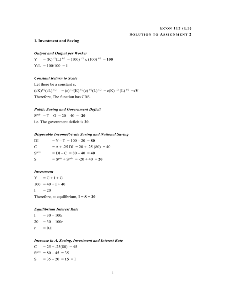
E C O N 11 2 ( L 5 )
SOLUTION TO ASSIGNMENT 2
1. Investment and Saving
Output and Output per Worker
Y
= (K)1/2(L) 1/2 = (100) 1/2 x (100) 1/2 = 100
Y/L = 100/100 = 1
Constant Return to Scale
Let there be a constant c,
(cK)1/2(cL) 1/2
= (c) 1/2(K) 1/2(c) 1/2(L) 1/2 = c(K) 1/2 (L) 1/2 =cY
Therefore, The function has CRS.
Public Saving and Government Deficit
Spub = T – G = 20 – 40 = -20
i.e. The government deficit is 20.
Disposable IncomePrivate Saving and National Saving
DI
= Y – T = 100 – 20 = 80
C
= A + .25 DI = 20 + .25 (80) = 40
Spriv
= DI – C = 80 – 40 = 40
S
= Spub + Spriv = -20 + 40 = 20
Investment
Y
=C+I+G
100 = 40 + I + 40
I
= 20
Therefore, at equilibrium, I = S = 20
Equilibrium Interest Rate
I
= 30 – 100r
20
= 30 – 100r
r
= 0.1
Increase in A, Saving, Investment and Interest Rate
C
= 25 + .25(80) = 45
Spriv = 80 – 45 = 35
S
= 35 – 20 = 15 = I
1
Therefore,
15
= 30 – 100r
r
= 0.15
Graphically,
I S1 S0
r
0.15
0.1
I,S
15
20
Saving function can be treated as the supply of fund while the investment function can be
treated as the demand. The exogenous variables of the model include output level, tax rate,
government spending, and consumption. The effects of the exogenous variables are
summarised as follows (ceteris paribus):
Variable
Effect to Saving
C
-ve
G
-ve
T
+ve
Y
+ve
The reduction in thriftness when A increases means there is an increase in consumption. With a
given level of output, the saving, and thus funds available for investment, decreases. The
interest rate therefore increases to restore the equilibrium of loan market.
Tax Increase and Change in Interest Rate
Zero budget deficit implies that public saving equal to zero, and that
T = G = 40 (i.e. increased by 20)
Then,
C
= 20 +.25(100 – 40) = 35
S
= (100 – 40) – 35 = 25
S
= 25 + 0 = 25 = I
priv
Therefore,
2
25
= 30 – 100r
r
= (30-25) / 100 = 0.05
By raising the tax, people’s disposable income, and thus private saving, decrease. The increase
in public saving is greater than the decrease in private saving. In some sense, the nation is
“forced” to save more in form of public saving. Investment in equilibrium thus increases as well.
The increase in investment then drives down the interest rate that clear the capital market.
2. Factor Prices and Technology Growth
Production Function
Yt  K t  Lt Et
Yt

Lt Et
~
yt 
K t  Lt Et
Lt Et
Kt
LE
~
~
 t t  kt 1  kt
Lt Et
Lt Et
The Steady State
I t  sYt
It
sYt

Lt Et Lt Et
~
~ ~
it  syt  0.2 k t
~
~
0.2 k t  (0.076  0.02  0.01)k t
~
k t  3.56
Therefore,
The graphical presentation of the steady state is given by
~
er(0.076  0.02  0.01)kt
~
0 .2 k t
~
kt
3.56
3
gY = n + gE = 0.02 + 0.01 = 0.03
gY/L = gE = 0.01
Factor Income Growth
At equilibrium, w=MPL. Therefore,
gw =gY-n = 0.03 – 0.02 = 0.01
Similar, r=MPK. Thus,
gr = gY – gK = gY –(n+gE) = 0.03 – 0.03 = 0
3. Labor Markets
Natural Rate of Unemployment
U t 1  (1  f )U t  sE t  rOt
U t 1  (1  f )U t  sE t  rOt
(U t 1  U t )  fU t  sE t  rOt
 fU t  sE t  qEt
fU t
E
 ( s  q) t
Lt
Lt
Ut
sq

Lt
f sq
In example 1,
Ut
0.01  0.01

 0.0909
Lt 0.2  0.01  0.01
In example 2,
Ut
0.01  0.05

 0.2308
Lt 0.2  0.01  0.05
i.e. When q increases, natural rate of unemployment increases.
When the teenagers’ quit rate is high in a country where teenagers makeup a large portion of the
labor force, q would be significantly high. From the above example, we can see that a higher
natural rate of unemployment will be resulted.
4