EE-371 CONTROL SYSTEMS LABORATORY
Session 3
State variable modeling and Introduction
to MATLAB Control System Toolbox
Purpose
The purpose of this session is to introduce the basics of state variable modeling known as
state-space techniques. The state-space technique is a unified time-domain formulation
that can be utilized for the analysis and design of linear and nonlinear continuous-time
and discrete-time multivariable systems. A short tutorial on the Basics of State-variable
Modeling will be presented in this session. The analytical solution of state equation will
be covered later in the lecture. Also, in this session few essential MATLAB Functions for
Modeling and Time-domain Analysis are introduced. After the above introductory
tutorial you will be able to complete the following two case studies.
Case Study 1
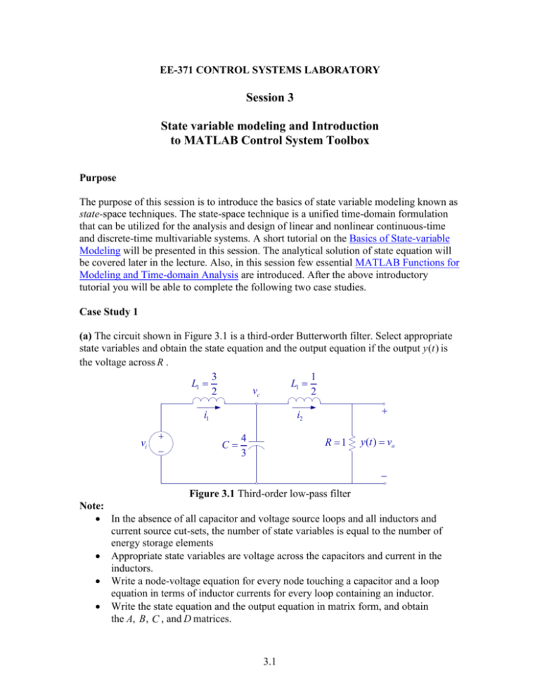
(a) The circuit shown in Figure 3.1 is a third-order Butterworth filter. Select appropriate
state variables and obtain the state equation and the output equation if the output y (t ) is
the voltage across R .
3
1
L1 
L1 
vc
2
2
i1
vi

i2
C
4
3
R 1
y (t )  vo

Figure 3.1 Third-order low-pass filter
Note:
 In the absence of all capacitor and voltage source loops and all inductors and
current source cut-sets, the number of state variables is equal to the number of
energy storage elements
 Appropriate state variables are voltage across the capacitors and current in the
inductors.
 Write a node-voltage equation for every node touching a capacitor and a loop
equation in terms of inductor currents for every loop containing an inductor.
 Write the state equation and the output equation in matrix form, and obtain
the A, B , C , and D matrices.
3.1
(b) Write a script m-file and use control system toolbox functions ss, and ltiview to form
the state model and its step response. Also, use ss2tf function to obtain the filter transfer
function. Run the m-file. Right-click on LTI Viewer and use Characteristics to display all
the time-domain specifications. From File menu select Print to Figure to obtain an
editable Figure plot. Next Right-click on the LTI Viewer and from the Plot Type list,
select Bode to obtain the Bode plot. Click on magnitude response, hold and drag to
display the corner frequency at –3.0 dB point. Also click on the magnitude response,
hold and drag to display the attenuation at 10 rad/s.
Summarize the step response characteristics and the filter transfer function. Comment on
the filter frequency response characteristics.
Case Study 2 — Moving-Coil Actuator
Linear and rotary moving-coil actuators are used for a wide variety of applications, such
as voice coil of loudspeakers, and for applications that require positioning over a small
range such as hard disk drives head positioning, laser beam mirror actuators, pen plotters,
and valve operators.
In its simplest form, a linear actuator is a tubular coil of wire placed within a permanent
magnet with uniform radial magnetic field B in the annular gap. The moving part has a
mass M and is assumed to have a viscous friction, which is shown externally by a dashpot
with frictional coefficient D . Also a spring restraining the motion with stiffness K is
considered as shown in Figure 3.2. The external forces due to the acceleration of mass,
frictional force and the spring force are acting against the magnetic force to hold the coil
in equilibrium. Note that x(t ) is the displacement and u (t ) is the velocity.
u (t )
x(t )
N
Coil
f (t )
S
N
Spring
K  40
Mass
M  0.4
Friction
D  4.48
i (t )
+v(t )
Figure 3.2 Moving coil actuator for Case Study 2
3.2
The current i (t ) is applied to the coil by means of flexible leads. The magnetic field
produced by the coil current interacts with the magnetic field of the permanent magnet,
which produces a force on the coil. The resulting force will cause the coil to move in or
out depending on the direction of current.
The Lorentz force law gives the magnitude of force
f (t )  Bli (t )  K f i (t )
(3.1)
When the coil is moving perpendicular to field with a velocity u (t ) , an emf is induced in
the coil in accordance to Faraday’s law
dx(t )
 Blu (t )  K eu (t )
(3.2)
dt
K f is in Newton/A and Ke is in V-s/m, their numerical values are the same given by
e(t )  Bl
K f  K e  Bl  B(2 rn)
(3.3)
where n is the number of turns of the coil and r is the coil radius.
The linear actuator shown has the following parameters:
Supply voltage
4 V dc
Coil inductance
L  80 mH
Coil resistance
R 8 .
Moving coil mass
M  0.4 Kg
Spring stiffness
K  40 N/m
Frictional coefficient
D  4.48 N-s/m
Permanent magnet flux density
B  0.51 Tesla
r  1 cm
Coil radius
Number of turns
n  50
2
K f  B(2 rn)  (0.51)(2 )(110 )(50)  1.6 N/A , and Ke  1.6 V-s/m
(a) Write the equation describing the electric circuit. Draw the force-voltage (or forcecurrent) electric circuit analogy for the mechanical system and write the equation
describing the mechanical system. Draw the s-domain block diagram for the
electromagnetic actuator with V ( s) as the reference input and the displacement X ( s) as
the output. (Mark all the s-domain variable V ( s) , I ( s ) , F ( s ) , U ( s ) , E ( s ) and X ( s) on
the block diagram and determine the transfer function X ( s ) / V ( s ) .
(b) Use MATLAB roots function to find the roots of the system transfer function and
determine the time constants. Obtain the electrical time constant  e  L / R and compare
to the mechanical time constant  m  1/ n  2M / D . If  e is small compared to  m ,
suggest a reduced-order model. Obtain the step response for the actual model and the
3.3
reduced-order model on the same graph. Once you have defined the numerators and
denominators for both systems, you can use sys3rd = tf(num1, den1), and
sys2nd = tf(num2, den2) to define the transfer function models. To obtain the step
response for both systems on the same LTI viewer use the following command
ltiview('step', sys3rd, 'b', sys2nd, 'r')
Right-click on the plot area and determine the time-domain characteristics, t r , t p , P.O. ,
and t s . Also the Bode magnitude plot can be obtained and compared to see that the
reduced-order model results in a very good match within the system bandwidth.
(c) The step response peak time and the percent overshoot of a second-order system is
given by
tp 

n 1   2

, and P.O.  e
1 2
100
(3.4)
Using the above relations compute t p , P.O. , and the settling time ( ts 4 ) for the
reduced-order model and compare to the values for the simulation response found in (b).
It can be shown that for linear actuators used for point-to-point applications with short
traveling distance, the maximum velocity attained is very small and for low Ke (V-s/m),
the back emf e(t )  Keu (t ) may be neglected. For this example in addition to neglecting
L if e(t ) is neglected, the transfer function with x(t ) in cm becomes
Kf
(100)
X ( s)
RM
G ( s) 

V (s) s 2  D s  K
M
M
3.4