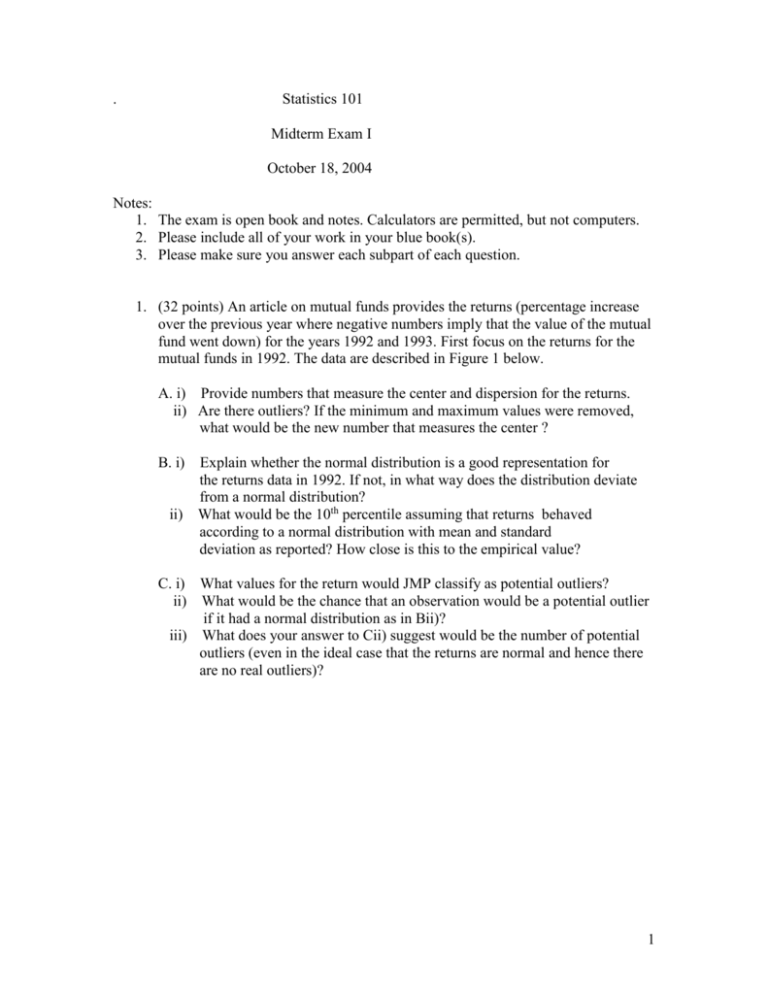
.
Statistics 101
Midterm Exam I
October 18, 2004
Notes:
1. The exam is open book and notes. Calculators are permitted, but not computers.
2. Please include all of your work in your blue book(s).
3. Please make sure you answer each subpart of each question.
1. (32 points) An article on mutual funds provides the returns (percentage increase
over the previous year where negative numbers imply that the value of the mutual
fund went down) for the years 1992 and 1993. First focus on the returns for the
mutual funds in 1992. The data are described in Figure 1 below.
A. i) Provide numbers that measure the center and dispersion for the returns.
ii) Are there outliers? If the minimum and maximum values were removed,
what would be the new number that measures the center ?
B. i)
Explain whether the normal distribution is a good representation for
the returns data in 1992. If not, in what way does the distribution deviate
from a normal distribution?
ii) What would be the 10th percentile assuming that returns behaved
according to a normal distribution with mean and standard
deviation as reported? How close is this to the empirical value?
C. i) What values for the return would JMP classify as potential outliers?
ii) What would be the chance that an observation would be a potential outlier
if it had a normal distribution as in Bii)?
iii) What does your answer to Cii) suggest would be the number of potential
outliers (even in the ideal case that the returns are normal and hence there
are no real outliers)?
1
Figure 1 Returns of Mutual Funds in 1992
Distributions
Return 92
60
50
40
30
20
10
0
-10
-20
-30
-40
-50
-60
.001 .01 .05.10 .25 .50 .75 .90.95 .99 .999
-4
-3
-2
-1
0
1
2
3
4
Normal Quantile Plot
Quantiles
100.0%
99.5%
97.5%
90.0%
75.0%
50.0%
25.0%
10.0%
2.5%
0.5%
0.0%
Maximum
Quartile
Median
Quartile
Minimum
57.83
39.63
22.73
15.96
9.96
7.94
5.53
0.038
-10.37
-21.63
-60.71
Moments
Mean
Std Dev
Std Err Mean
upper 95% Mean
lower 95% Mean
N
7.6917873
7.9009323
0.2017935
8.0876081
7.2959666
1533
2
D. The mean and standard deviation of the returns in 1993 are found to be 14.86 and
13.68 respectively. The correlation between 1992 and 1993 returns is -.2835.
i) What fraction of the variability of returns in 1993 is accounted for by the returns in
1992?
ii) What would be the predicted return in 1993 for the most promising mutual fund in
1992 (i.e., the one with return of 57.83%)?
2. (24 points) Seismology data collected from all over the world show quite clearly that
the average number of shocks per year, Y, is related to the severity, X, of earthquakes in
units on the Richter scale. The following data are collected in southern California:
X: 4.0 4.5 5.0 5.5 6.0 6.5 7.0
Y:33.0 11.5 3.4 1.4 0.5 0.2
.09
Refer to Figure 2a below in answering Part A. A regression is run to predict the number
of shocks per year Y, from the severity, X.
A. i) What is the predicted number of shocks per year at a severity level of 8.0 on
the Richter scale?
ii) Be specific as to the output you are relying on in commenting on whether this
analysis is appropriate
3
Figure 2a Shocks per year by severity
Biv a riate Fit of Shoc ks /yr By Se v e rity
Shocks/yr
40
30
20
10
0
3
4
5
6
7
8
Severity
Linear Fit
Linea r Fit
Shocks/yr = 55.960357 - 8.8735714
Severity
Summary of Fit
RSquare
RSquare Adj
Root Mean Square Error
Mean of Response
Observations (or Sum Wgts)
0.628745
0.554494
8.067918
7.155714
7
Para me te r Estimate s
Term
Intercept
Severity
Estimate
Std Error
t Ratio
55.960357
-8.873571
17.04659
3.049386
3.28
-2.91
Prob>| t|
0.0219
0.0334
Residual
15
10
5
0
-5
-10
3
4
5
6
7
8
Severity
B. Figure 2b provides the output for predicted natural log of frequency versus
severity.
i) What is the predicted number of shocks per year at a severity level of 8?
ii) How likely would it be for the number of shocks per year to exceed .0125 (that is
once in 80 years) at a severity level of 8?
Hint: If the number of shocks per year is to exceed .0125, what does that imply about
the natural logarithm of the number of shocks per year?
4
Figure 2b Natural log of Shocks per year by severity
Biv a riate Fit of Shoc ks /yr By Se v e rity
Shocks/yr
40
30
20
10
0
3
4
5
6
7
8
Severity
Transformed Fit Log
Tra ns formed Fit Log
Log(Shocks/yr) = 11.293809 - 1.9809894
Severity
Summary of Fit
RSquare
RSquare Adj
Root Mean Square Error
Mean of Response
Observations (or Sum Wgts)
0.99676
0.996112
0.133641
0.398367
7
Para me te r Estimate s
Term
Intercept
Severity
Estimate
Std Error
t Ratio
11.293809
-1.980989
0.282368
0.050512
40.00
-39.22
Prob>| t|
<.0001
<.0001
Fit Me as ure d on Original Sc a le
Residual
Sum of Squared Error
Root Mean Square Error
RSquare
Sum of Residuals
16.288177
1.8048921
0.9814197
3.8832776
5
4
3
2
1
0
-1
3
4
5
6
7
8
Severity
C i) Which model fits better, the one in part A or in part B? Write a few sentences
supporting your answer.
ii) Are you satisfied with that model you chose in part Ci)? If yes, explain. If not,
indicate what modification(s) you would make and why.
5
3. (28 points) An analysis is performed to predict the price of diamonds (in Singapore
dollars). Clearly the price of a diamond depends on its weight. A regression is run with
this aim. The results appearing in Figure 3a.
Ai) Explain carefully what the value of the slope means in the context of this problem.
ii) Based on the results below, do you have any issues with the analysis? Be specific.
Bi) Someone is selling a diamond that weighs .25 carats for $700. Is this a good deal?
Explain.
ii) Based on the results below (and the assumption of normality), what proportion of
diamonds of .25 carats would sell for more than $700?
Figure 3a Price of diamonds versus weight
Price (Singapore dollars)
Bivariate Fit of Price (Singapore dollars) By Weight (carats)
1100
1000
900
800
700
600
500
400
300
200
.1
.15
.2
.25
.3
.35
Weight (carats)
Linear Fit
Linear Fit
Price (Singapore dollars) = -259.6259 +
3721.0249 Weight (carats)
Summar y of Fit
RSquare
RSquare Adj
Root Mean Square Error
Mean of Response
Observations (or Sum Wgts)
0.978261
0.977788
31.84052
500.0833
48
Parameter Estimates
Term
Intercept
Weight (carats)
Estimate
Std Error
t Ratio
-259.6259
3721.0249
17.31886
81.78588
-14.99
45.50
Prob>| t|
<.0001
<.0001
Residual
100
50
0
-50
-100
.1
.15
.2
.25
.3
.35
Weight (carats)
6
C. The price of diamonds depends not only on its size, but also on its clarity. The
residuals are saved from the regression of Y (price) versus X (weight). These
residuals are then analyzed below in Figure 3b by fitting Y (residuals) versus X
(clarity).
i) What would you expect the average residual to be for each level of clarity if
clarity had no effect?
ii) It is decided to adjust the prediction in the regression in Figure 3a either up or
down by adding the average residual for the level of clarity. Would this be a
reasonable thing to do if the average increase in price per unit increase in
weight depended on clarity? Explain.
D. Does the model that adjusts for clarity (by adding the average residual for the
appropriate level of clarity) predict prices for diamonds more accurately than
the model that ignores clarity? Explain.
Figure 3b Residuals of the regression on Clarity
Residuals Price (Singapore dollars) 2
Onew ay Analysis of Residuals Price (Singapore dollars) 2 By Clarity
100
50
0
-50
-100
High
Low
Middle
Clarity
Means and Std Dev iations
Level
High
Low
Middle
Number
Mean
Std Dev
Std Err Mean
Lower 95%
Upper 95%
13
14
21
36.105
-28.613
-3.276
20.1230
23.3127
17.4319
5.5811
6.2306
3.8040
23.95
-42.07
-11.21
48.27
-15.15
4.66
7
4. (16 points) A survey is taken of 810 individuals, to see what age is the best to
market to in promoting a new palm pilot. The results of the survey are
summarized below in Figure 4a.
A. i) Based on the results reported in Figure 4a, explain briefly what age
group appears to be the best target market in terms of having the largest
proportions of buyers.
ii) It is realized that the survey was done randomly within age group, but in
the upper age group more individuals were chosen than reflected in the
population. In fact, the low aged people represent 40%, the middle aged
40% and upper aged 20% of the population. If the criterion to be used is
the proportion of buyers in each age group, how, if at all, would your
answer to i) change?
iii) If the criterion to be used is number of potential buyers in the age
group, what would you suggest is the best test market taking into account
the true population proportions for the age groups as indicated in ii).
Figure 4a. Age versus likelihood of buying
Contingency Table
Age
Buy
Count
NO
YES
Total %
Col %
Row %
LOW
208
65
25.68
8.02
35.02
30.09
76.19
23.81
MIDDLE
208
72
25.68
8.89
35.02
33.33
74.29
25.71
UPPER
178
79
21.98
9.75
29.97
36.57
69.26
30.74
594
216
73.33
26.67
273
33.70
280
34.57
257
31.73
810
8
B. It is decided to get a more refined look at who is likely to purchase the new
palm pilot, income should also be included in the analysis. Figures 4b, 4c and
4d redo the analysis for low income, middle income and upper income
respectively.
Assume as in Ai) that the criterion is to find the subpopulation that has the
largest proportion of potential buyers. Also ignore the fact that the survey
might have favored certain age groups over other age groups. Comment on
the best age group within each of the three income classes.
Compare your answers in B with Ai) and explain whether income is changing
the picture and why. Be specific.
Figure 4b. Age versus likelihood of buying for low income individuals
Contingency Table
Age
Buy
Count
NO
YES
Total %
Col %
Row %
LOW
130
32
43.05
10.60
51.18
66.67
80.25
19.75
MIDDLE
87
13
28.81
4.30
34.25
27.08
87.00
13.00
UPPER
37
3
12.25
0.99
14.57
6.25
92.50
7.50
254
48
84.11
15.89
162
53.64
100
33.11
40
13.25
302
9
Figure 4c. Age versus likelihood of buying for middle income individuals
Age
Contingency Table
Buy
Count
NO
YES
Total %
Col %
Row %
LOW
73
25
23.93
8.20
30.17
39.68
74.49
25.51
MIDDLE
88
23
28.85
7.54
36.36
36.51
79.28
20.72
UPPER
81
15
26.56
4.92
33.47
23.81
84.38
15.63
242
63
79.34
20.66
98
32.13
111
36.39
96
31.48
305
Figure 4d. Age versus likelihood of buying for upper income individuals
Contingency Table
Buy
Count
NO
Total %
Col %
Row %
LOW
Age
MIDDLE
UPPER
5
2.46
5.10
38.46
33
16.26
33.67
47.83
60
29.56
61.22
49.59
98
48.28
YES
8
3.94
7.62
61.54
36
17.73
34.29
52.17
61
30.05
58.10
50.41
105
51.72
13
6.40
69
33.99
121
59.61
203
10