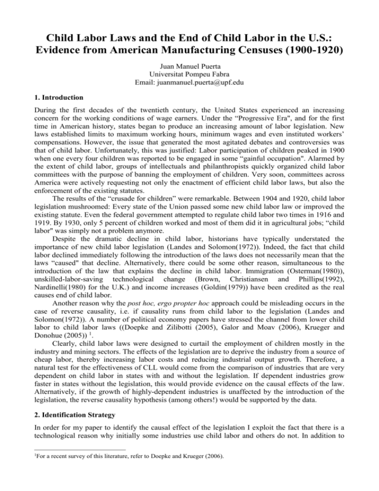
Child Labor Laws and the End of Child Labor in the U.S.:
Evidence from American Manufacturing Censuses (1900-1920)
Juan Manuel Puerta
Universitat Pompeu Fabra
Email: juanmanuel.puerta@upf.edu
1. Introduction
During the first decades of the twentieth century, the United States experienced an increasing
concern for the working conditions of wage earners. Under the “Progressive Era", and for the first
time in American history, states began to produce an increasing amount of labor legislation. New
laws established limits to maximum working hours, minimum wages and even instituted workers’
compensations. However, the issue that generated the most agitated debates and controversies was
that of child labor. Unfortunately, this was justified: Labor participation of children peaked in 1900
when one every four children was reported to be engaged in some “gainful occupation". Alarmed by
the extent of child labor, groups of intellectuals and philanthropists quickly organized child labor
committees with the purpose of banning the employment of children. Very soon, committees across
America were actively requesting not only the enactment of efficient child labor laws, but also the
enforcement of the existing statutes.
The results of the “crusade for children” were remarkable. Between 1904 and 1920, child labor
legislation mushroomed: Every state of the Union passed some new child labor law or improved the
existing statute. Even the federal government attempted to regulate child labor two times in 1916 and
1919. By 1930, only 5 percent of children worked and most of them did it in agricultural jobs; “child
labor" was simply not a problem anymore.
Despite the dramatic decline in child labor, historians have typically understated the
importance of new child labor legislation (Landes and Solomon(1972)). Indeed, the fact that child
labor declined immediately following the introduction of the laws does not necessarily mean that the
laws “caused" that decline. Alternatively, there could be some other reason, simultaneous to the
introduction of the law that explains the decline in child labor. Immigration (Osterman(1980)),
unskilled-labor-saving technological change (Brown, Christiansen and Phillips(1992),
Nardinelli(1980) for the U.K.) and income increases (Goldin(1979)) have been credited as the real
causes end of child labor.
Another reason why the post hoc, ergo propter hoc approach could be misleading occurs in the
case of reverse causality, i.e. if causality runs from child labor to the legislation (Landes and
Solomon(1972)). A number of political economy papers have stressed the channel from lower child
labor to child labor laws ((Doepke and Zilibotti (2005), Galor and Moav (2006), Krueger and
Donohue (2005)) 1.
Clearly, child labor laws were designed to curtail the employment of children mostly in the
industry and mining sectors. The effects of the legislation are to deprive the industry from a source of
cheap labor, thereby increasing labor costs and reducing industrial output growth. Therefore, a
natural test for the effectiveness of CLL would come from the comparison of industries that are very
dependent on child labor in states with and without the legislation. If dependent industries grow
faster in states without the legislation, this would provide evidence on the causal effects of the law.
Alternatively, if the growth of highly-dependent industries is unaffected by the introduction of the
legislation, the reverse causality hypothesis (among others!) would be supported by the data.
2. Identification Strategy
In order for my paper to identify the causal effect of the legislation I exploit the fact that there is a
technological reason why initially some industries use child labor and others do not. In addition to
1
For a recent survey of this literature, refer to Doepke and Krueger (2006).
this, I need that the CLL are exogenous to the industries. This could be argued on the grounds that
the legislation was mostly sponsored by phylantropic organizations and that, in any case, most of
industries in my sample are far too small to influence the state political process.
The outcome variables I will be considering is the real value added growth, measured as the
compouded annualized rate of growth. The basic model I will estimate in this paper is then
Y j  s     0 X j  s  1U i   2Vs  3CLLs  CL Dependence j   j s
(1)
where Y j  s is the chosen outcome variable. X j  s includes the variables other than the
interaction that vary at both state and industry level like industry size in the state; or the proportion of
total value added produced by industry j in the state s. U j contains the initial dependence on child
labor to be defined later. Finally Vs includes a whole set of controls for state specific characteristics
such as illiteracy rate, state investment, initial income per capita and a whole set of demographic
controls.
Child Labor Dependence is an industry-level variable indicating the degree to which industry
j used child labor when there were not any restrictions to child labor employment. The CLL dummy
indicates whether state s has a child labor law enacted at the period. This interaction represents the
extent to which the combination of Child Labor Dependence and Child Labor Law Dummy depresses
growth and is the variable of interest in this study.
3. Main Results
In this section I present the results of my estimation of equation (1) above. I try four alternative
specifications including a number of state and industry controls. In the final specification I
concentrate on the interaction term alone and allow for a full set of industry and state controls. The
results are presented in Table 1.
Ln. Wage Earners
Table 1: Basic Specification
(1)
(2)
0.004
0.01
(0.002)
(0.003)***
(3)
0.003
(0.004)
(4)
0.016
(0.006)***
0.007
(0.004)
Ln. Real Capital
0.005
(0.002)**
0.012
(0.003)***
0.002
(0.004)
Prop. Manufacturing
-.012
(0.002)***
-.026
(0.005)***
-.013
(0.002)***
CL Dependence
0.327
(0.067)***
-.0003
(0.005)
0.303
(0.068)***
CLL
State Investment
1900-10
Black (%)
Urban (%)
Illiteracy(%)
0.004
(0.004)
0.02
0.019
(0.007)***
(0.005)***
0.119
(0.041)***
-.038
(0.02)*
0.143
(0.035)***
-.034
(0.017)**
-.082
(0.092)
-.131
(0.077)*
-.030
(0.006)***
Foreign (%)
Ln. Patents
Ln. State Income 1900
CLL&Dependence
N
0.005
(0.036)
0.003
(0.009)
0.007
(0.029)
0.005
(0.008)
0.019
(0.012)
0.016
(0.011)
-.301
(0.106)***
2154
-.304
(0.104)***
2194
-.248
(0.096)***
2154
-.232
(0.094)**
2194
R2
0.043
0.074
0.427
0.458
Industry Dummies
NO
NO
YES
YES
State Dummies
NO
YES
NO
YES
Note: OLS coefficients from regression 1 in the text. Dependent variable: Annual Compounded growth rate of
value added for the period 1910-1920. Robust standard errors in parenthesis. *,**,*** denote 10,5 and 1 percent
significance respectively. Unless otherwise specified, all the variables correspond to 1910. CLL refers to “effective”
child labor laws, that is, child labor laws combined with factory inspection and compulsory schooling. CL dependence
is the median proportion of children employed industry-wise in 1900.
The coefficient of interest is the interaction between child labor dependence and CLL. This
interaction is similar to a second derivative: the differential effect of a child labor law for industries
that are highly dependent in child labor compared with those that are not. The point estimates for the
interaction of child dependence and child labor laws range between -0.2 and -0.3 and they are
significant at conventional level. Their effect on growth rates will depend on the percentage of
children initially employed. For the average firm, employing about 2 percent of children, this effect
could imply a decline in growth of the order of 0.4 to 0.6 percentage points per year. The other
variables I include in the first regression have interesting and plausible signs. In particular, the
proportion of urban and black population, and state income are all proxying for the initial level of
development, which explains their signs.
In general econometric terms specification (1)-(4) looks good. The interaction coefficient is
surprising stable across specifications. This is interesting as the number of controls used in each of
the regressions varies dramatically. In the baseline case, a full set of 153 industry dummies and 48
state dummies are included. This contrasts with the mere 13 controls included in specification (1). In
spite of these differences, the effect on the coefficient is mild, not affecting its statistical significance.
The explanatory power of the regression ( R2 ) raises significantly after the introduction of a full set
of industry dummies. This result just suggests that most of the variation in annual growth rates of
industries have to do with omitted industry-specific characteristics. More importantly for my
argument, the negative and significant effect subsists even when I control for industry-specific
growth.
4. Robustness
Obviously industries may vary across the different states for a number of reasons other than their
child labor dependence at the beginning of the period. In this section, I perform a number of
robustness checks in order to rule out other alternative explanations. First, I check whether the results
are sensitive to the definition of child labor dependence. In order to do so, I construct a child labor
dependence based on children employement in census dates before 1900. Failure to find an effect of
child labor dependence so defined would cast doubt about the universality of my results.
After proving the robustness of the results with respect to the dependence measure in Table 2, I
turn my attention to the definition of child labor laws. I consider alternative specifications including
a plain dummy for CLL, this dummy interacted with the working permit requirement or the
compulsory schooling requirement. Again, the results of Table 3 show that the effect is there even if
we define the child labor law in a slightly different way.
Another set of robustness checks (Table 4) restricts the sample according to the initial level of
child labor dependence or the initial relative size of the industry. In principle, only industries that
were initially employing children should be affected by the laws. On the other hand, in order to deal
with political economy concerns, I restrict the analysis to small industries. Arguably, even if the laws
were self-imposed once children were not necessary in the industry, this should hold true only in
large industries capable of lobbying for a law. Small industries simply received the legislative shock
exogenously.
Finally, I try alternative estimation procedures (Table 4) that are more robust to aberrant
observations. These estimation procedures are based on the median (LAD) or on a recursive
weighted OLS procedure (Robust regression). Again, although the results are smaller, the general
findings are confirmed.
Ln. Wage
Earners
Ln. Real Capital
Prop.
Manufacturing
Children
1880&CLL
Table 2: Other CL Dependence Measures
(1)
(2)
0.017
0.013
(4)
0.011
(0.006)***
(0.006)**
(0.006)***
(0.006)*
0.007
(0.005)
0.005
(0.005)
0.007
(0.004)
0.006
(0.005)
-.032
-.022
-.031
-.022
(0.007)***
(0.006)***
(0.006)***
(0.007)***
-.084
-.106
(0.057)
(0.065)*
-.156
-.210
(0.092)*
(0.11)*
2194
2194
Children
1890&CLL
N
(3)
0.016
2057
2057
2
R
0.459
0.457
Note: General notes apply (see Table 1). Columns 1and 3 estimated by OLS with robust standard errors.
Median regression coefficients with bootstrapped standard errors (200 reps.) reported in columns 2 and 4.
Table 3:Other CLL Laws
(1)
(2)
Ln. Wage
Earners
0.016
0.016
(0.006)***
(0.006)***
(3)
0.016
(0.006)
***
Ln. Real Capital
Prop.
Manufacturing
0.007
(0.004)
0.007
(0.004)
-.031
-.031
(0.006)***
(0.006)***
0.007
(0.004)
-.031
(0.006)
***
CLL Alone
(4)
0.016
(0.005)*
**
0.007
(0.004)
-.032
(0.006)*
**
-.130
(0.088)
CLL&Papers
-.188
(0.093)**
CSL Alone
-.157
(0.089)
*
CLL
N
R2
2194
0.457
2194
0.457
2194
0.457
-.247
(0.095)*
**
2142
0.463
But NC
&SC
Note: General notes apply (see Table 1). CSL stands for “Compulsory schooling laws”.
CLL&Papers stands for the child-labor ban combined with a working paper (not affidavit) requirement.
CLL Alone stands for the simple child labor law with no additional requirement,.
Sample
Ln. Wage
Earners
Ln. Real
Capital
Prop.
Manufacturing
CL
Dependence&CLL
ALL
(1)
0.016
ALL
Table 4:Other Robustness Checks
(2)
0.022
ALL
(3)
0.012
(0.006)**
(0.007)***
(0.005)**
0.002
0.005
0.006
(0.005)
(0.006)
(0.005)
-.023
-.044
-.022
(0.007)***
(0.008)***
(0.008)***
-.270
-.314
-.157
(4)
0.012
(0.004)***
0.006
(0.003)**
-.023
(0.004)***
-.160
(0.102)***
(0.138)**
(0.091)*
(0.093)*
1609
1434
2194
2194
0.457
0.474
0.495
OLS
OLS
LAD
Robust
CL Dep >
P ropManuf <
Sample
W hole
W hole
0
1%
Note: General notes apply (see Table 1). Robust standard errors for specifications (1) and (2).
Bootstrapped standard errors (20 reps.) in specifications (3). Specification (4) is a regression where
observation with large residuals are reweighted in order to attenuate their impact (robust regression,
Huber(1964)). Bi-weights set to 8 times the median absolute deviation from the median residual.
N
R2
Est. Method
5. Conclusion
This paper examines the consequences of the child labor legislation on the manufacturing sector of
the United States. Examining this case is interesting for various reasons. From purely historical
reasons, child labor legislation offers a unique example of a resounding public policy whose
effectiveness has been questioned. In addition to this, the study of the implementation and economic
consequences of a historical child labor law may be important in order to understand the difficulties
of eradicating child labor in the developing economies of today.
I find out that CLL have a deletorious and potentially big effect on industrial growth. This
effect ranged from a negligible growth effect to over 1 percent per year for industries employing
children extensively. These results are both plausible and consistent with the behavior of industries:
Rather than enjoying the ride after the CLL got passed, as the modern political-economy models
would suggest, industries fought fiercely against the ban.
Other than to shed some light into the issue of child labor and the effect of legislation, this
paper contributes to the literature in at least two other ways. First, I use a previously unexploited
source of data (U.S. manufacturing census) in order to give a novel answer to the question of child
labor in America.
Second, my methodology is inspired on a very well-known methodology of the development
economics literature. In particular, I identify a channel through which child labor laws should affect
some industries more than other. Exploiting this source of variation, I go around reverse causality
issues at a state level. This is so because it is possible for me to compare industries that received the
shock and those that did not within the same state. In a word, this methodology allows me to
conclude that it is not the growth rate that explains the law, but rather the law explaining the growth
rate.
References
BROWN, M., J. CHRISTIANSEN, AND P. PHILLIPS (1992): “The Decline of Child Labor in
the U.S. Fruit and Vegetable Canning Industry: Law or Economics?,” Business History Review,
66(4), 723–770.
DOEPKE, M., AND D. KRUEGER (2006): “Origins and Consequences of Child Labor
Restrictions:A Macroeconomic Perspective,” NBER Working Papers 12665, National Bureau of
Economic Research.
DOEPKE, M., AND F. ZILIBOTTI (2005): “The Macroeconomics of Child Labor
Regulation,” American Economic Review, 95(5), 1492–1524.
EASTERLIN, R. A. (1957): "State Income Estimates" in Everett S. Lee, Ann Ratner Miller,
Carol Brainerd, and Richard A. Easterlin, Population Redistribution and Economic Growth: United
States 1870-1950, Vol. 1 (Philadelphia: The American Philosophical Society), 701-759.
EDWARDS, L. N. (1978): “An Empirical Analysis of Compulsory Schooling Legislation,
1940-1960,” Journal of Law & Economics, 21(1), 203–22.
GALOR, O., AND O. MOAV (2006): “Das Human Kapital: A Theory of the Demise of the
Class Structure,” Review of Economic Studies, 73(1), 85–117.
GOLDIN, C. (1979): “Household and market production of families in a late nineteenth
century American city,” Explorations in Economic History, 16(2), 111–131.
HAINES, M. R., AND ICPSR (2004): “Historical, Demographic, Economic and Social Data:
The United States 1790-2000,” Computer File.
HINDMAN, H. D. (2002): Child Labor. An American History. M.E. Sharpe.
JOHNSON, D. (2002): “U.S. Historical Patent Set (USHiPS),” Computer File.
KRUEGER, D., AND J. T. DONOHUE (2005): “On The Distributional Consequences Of
Child Labor Legislation,” International Economic Review, 46(3), 785–815.
KRUSE, D., AND D. MAHONY (1998): “Illegal Child Labor in the United States: Prevalence
and Characteristics,” NBER Working Papers 6479, National Bureau of Economic Research.
LANDES, W., AND L. C. SOLMON (1972): “Compulsory Schooling Legislation: An
Economic Analysis of Law and Social Change in the Nineteenth Century,” The Journal of Economic
History, 32(1), 54–91.
MARGO, R. A., AND T. A. FINEGAN (1996): “Compulsory Schooling Legislation and
School Attendance in Turn-of-the-Century America: A ’Natural Experiment’ Approach,” Economic
Letters, 53, 103–110.
MOEHLING, C. M. (1999): “State Child Labor Laws and the Decline of Child Labor,”
Explorations in Economic History, 36(1), 72–106.
NARDINELLI, C. (1980): “Child Labor and the Factory Acts,” The Journal of Economic
History, 40(4), 739–755.
OGBURN, W. F. (1968): Progress and Uniformity in State Child Labor Legislation: A Study
in Statistical Measurement. AMS Press.
OSTERMAN, P. (1980): Getting Started: The Youth Labor Market. The MIT Press.
RAJAN, R. G., AND L. ZINGALES (1998): “Financial Dependence and Growth,” American
Economic Review, 88(3), 559–86.
SANDERSON, A. R. (1974): “Child-Labor Legislation and the Labor Force Participation of
Children,” Journal of Economic History, 34(1), 297–299.