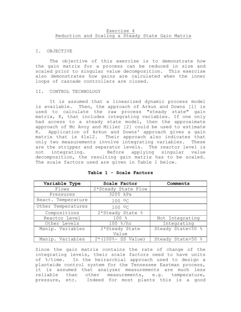
Exercise 4
Reduction and Scaling a Steady State Gain Matrix
I.
OBJECTIVE
The objective of this exercise is to demonstrate how
the gain matrix for a process can be reduced in size and
scaled prior to singular value decomposition. This exercise
also demonstrates how gains are calculated when the inner
loops of cascade controllers are closed.
II.
CONTROL TECHNOLOGY
It is assumed that a linearized dynamic process model
is available. Then, the approach of Arkun and Downs [1] is
used to calculate the raw process "steady state" gain
matrix, K, that includes integrating variables. If one only
had access to a steady state model, then the approximate
approach of Mc Avoy and Miller [2] could be used to estimate
K.
Application of Arkun and Downs' approach gives a gain
matrix that is 41x12.
Their approach also indicates that
only two measurements involve integrating variables. These
are the stripper and separator levels. The reactor level is
not
integrating.
Before
applying
singular
value
decomposition, the resulting gain matrix has to be scaled.
The scale factors used are given in Table 1 below.
Table 1 - Scale Factors
Variable Type
Flows
Pressures
React. Temperature
Other Temperatures
Compositions
Reactor Level
Other Levels
Manip. Variables
Manip. Variables
Scale Factor
2*Steady State Flow
3200 kPa
100 oC
100 oC
2*Steady State %
100 %
100 %/hr
2*Steady State
Value
2*(100%- SS Value)
Comments
Not Integrating
Integrating
Steady State<50 %
Steady State>50 %
Since the gain matrix contains the rate of change of the
integrating levels, their scale factors need to have units
of %/time.
In the heirarchial approach used to design a
plantwide control system for the Tennessee Eastman process,
it is assumed that analyzer measurements are much less
reliable
than
other
measurements,
e.g.
temperature,
pressure, etc.
Indeed for most plants this is a good
assumption to make. A byproduct of making this assumption
is that the resulting control system should be the best
possible if for some reason the analyzer becomes inoperable.
In this exercise only the non-analyzer loops are considered.
The
non-analyzer
measurements
involve
the
first
22
measurements, and thus only the first 22 rows of the raw
"steady state" gain matrix are used.
Eliminating the
analyzer gives a 22x12 gain matrix. Ten of the rows of the
resulting 22x12 matrix involve the gains for the inner loops
of the cascade controllers that will be closed.
These
variables are shown in Table 2 below.
Table 2 - Inner Cascade Measurements
Measurement
Row Number
A Flowrate
D Flowrate
E Flowrate
C Flowrate
Purge Flowrate
Separator Exit Flow
Product Flowrate
Steam Flowrate
React.CW
Outlet
Temp
React.CW
Outlet
Temp
1
2
3
4
10
14
17
19
21
Manipulated
Variable
3
1
2
4
6
7
8
9
10
22
11
The inner cascade measurements can be eliminated serially as
follows.
First start with the A Flowrate, which involves
measurement 1 and manipulated variable 3. The initial 22x12
gain matrix can be written as:
xmeas  K *u
(1)
If xmeas for the flowrate of A is set to FAset then the
first row of eqn. 1 can be solved for u3, the signal going
to the A valve, as:


12
set

u3  F A   K1, ju j 
 / K1,3
j1


j 3
(2)
Using eqn. 2 one can eliminate u3 as a manipulated variable
in favor of FAset .
Elimination of u3 gives a new gain
matrix whose elements are:
Ki, j  Ki, j  Ki, 3 * K1, j / K1,3
/
j 3
(3)
Ki,3 /  Ki,3 / K1,3
and
u / 
u  FAset 
 
u / / 
(4)
where u' and u'' contain all the original manipulated
variables, except u3. Since u3 has been eliminated in favor
of FAset , the dimension of K' is 22x12 and its third column
gives the gain elements for manipulating FAset . The first
row of K' has zeros in every column except the column
associated with u3 which has a 1. In the computer exercise,
the correct column for a manipulated variable can be
determined by examining the MATLAB variable, Glabel (for
gain label).
Next the D flowrate can be eliminated by
taking the same approach as was done for A, but now using
the K' matrix.
In this manner each of the inner cascade
measurements can be eliminated one at a time.
If
variable
then the
rows are
III.
all the rows that involve the cascade set point
affecting itself with a unity gain are eliminated,
resulting gain matrix is reduced to 12x12, i.e. the
reduced by 22 minus 10 cascaded measurements.
COMPUTER EXERCISE
This exercise involves the use of a number of MATLAB
routines. First the raw gain matrix, K, can be loaded into
memory using the mat-file TEgain.mat.
K is the 41x12 raw
gain matrix.
Labels can be determined for the rows and
columns of K by calling the m-file Glabel=gainlbl. Glabel
is a 42 row array which has a header and which gives all the
measurements and manipulated variables. The raw gain matrix
can be scaled by calling the m-file k=scale(K,u,zs), with
the scaled gain matrix, k, returned. Before calling scale
the mat file steady needs to be loaded. At this point rows
23 to 41 (analyzer rows) can be eliminated from k and rows
24 to 42 can be eliminated from Glabel by a simple MATLAB
command (k=k(1:22,:), and Glabel=Glabel(1:23,:)). To carry
out
the
serial
elimination
of
the
inner
cascade
measurements, the m-file, [kp,Glabel]= cascade1(k,Glabel),
can be used.
This m-file asks which cascade manipulated
variable, m, is being considered, and it returns kp, the
gain matrix resulting from closing the cascade loop on the
measurement of m's effect (a flowrate, or temperature). Be
careful with inputs and outputs to the cascade1 m-file so
that you don't erase an earlier result. The input k needs
to be set to kp after each cascade loop is closed.
The
matrix of labels, Glabel, is updated by cascade1. The final
12x12 scaled gain matrix can be calculated by calling the mfile, [k,Glabel]=elim(k,Glabel), which eliminates the rows
associated with the inner cascade measurements.
IV.
EXERCISES
Exercise 1. Load the raw gain matrix for the process,
TEgain.mat.
Display the gain labels using
gainlbl.
Scale the raw gain matrix using
scale, and eliminate rows 23 to 41 in the
scaled matrix, k, as well as rows 24 to 42 in
the label matrix, Glabel.
Exercise 2.
Starting with the scaled gain matrix for the
non-analyzer variables, eliminate the inner
cascade measurements, shown in Table 2, using
cascade1. As each variable is eliminated check
its associated row.
Exercise 3. Eliminate the rows associated with the inner
cascade measurements using elim.
V.
RESULTS ANALYSIS
After all the inner cascades are eliminated, verify
that the rows associated with all inner cascade loops form a
perturbed version of an identity matrix.
What does this
result tell you about the process of closing cascade loops?
Compare your final 12x12 gain matrix to that given in the
mat-file TEresult. If the cascade variables (yc, uc) and the
non-cascade variables (y, u) are separated in the original
gain matrix as:
yc  AC , A12  uC 


y 
 
A21 , A22 
 
u 

develop a general expression for the gain matrix
results from closing the inner cascade controllers.
VI. REFERENCES:
(5)
that
[1]
Arkun, Y. and J. Downs, "A General Method to Calculate
Input-Output Gains and the Relative Gain Array for
Integrating Processes," Computers Chem. Engng., 14(10),
1101-1110 (1990).
[2]
Mc Avoy, T., and Miller, R., "Incorporating Integrating
Variables Into Steady State Models For Plantwide
Control Analysis and Design", I&EC Research, 38, pp.
412-420 (1999).