CHAPTER 2
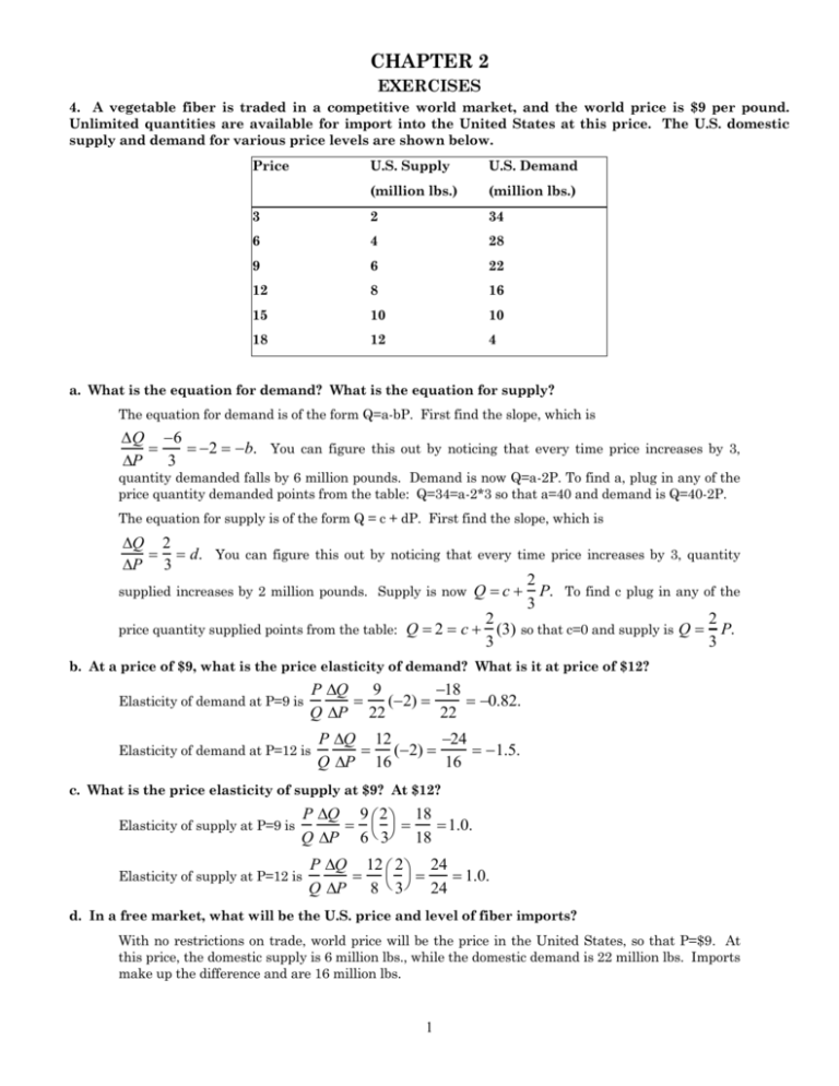
EXERCISES
4. A vegetable fiber is traded in a competitive world market, and the world price is $9 per pound.
Unlimited quantities are available for import into the United States at this price. The U.S. domestic
supply and demand for various price levels are shown below.
Price
U.S. Supply
U.S. Demand
(million lbs.)
(million lbs.)
3
2
34
6
4
28
9
6
22
12
8
16
15
10
10
18
12
4
a. What is the equation for demand? What is the equation for supply?
The equation for demand is of the form Q=a-bP. First find the slope, which is
Q 6

 2  b. You can figure this out by noticing that every time price increases by 3,
P
3
quantity demanded falls by 6 million pounds. Demand is now Q=a-2P. To find a, plug in any of the
price quantity demanded points from the table: Q=34=a-2*3 so that a=40 and demand is Q=40-2P.
The equation for supply is of the form Q = c + dP. First find the slope, which is
Q 2
  d. You can figure this out by noticing that every time price increases by 3, quantity
P 3
2
supplied increases by 2 million pounds. Supply is now Q  c  P. To find c plug in any of the
3
2
2
price quantity supplied points from the table: Q  2  c  (3) so that c=0 and supply is Q  P.
3
3
b. At a price of $9, what is the price elasticity of demand? What is it at price of $12?
Elasticity of demand at P=9 is
P Q
9
18

(2) 
 0.82.
Q P 22
22
Elasticity of demand at P=12 is
P Q 12
24
 (2) 
 1.5.
Q P 16
16
c. What is the price elasticity of supply at $9? At $12?
Elasticity of supply at P=9 is
P Q 9 2  18


 1.0.
Q P 6 3 18
Elasticity of supply at P=12 is
P Q 12 2  24


 1.0.
Q P 8 3  24
d. In a free market, what will be the U.S. price and level of fiber imports?
With no restrictions on trade, world price will be the price in the United States, so that P=$9. At
this price, the domestic supply is 6 million lbs., while the domestic demand is 22 million lbs. Imports
make up the difference and are 16 million lbs.
1
7. In 1998, Americans smoked 470 billion cigarettes, or 23.5 billion packs of cigarettes. The average
retail price was $2 per pack. Statistical studies have shown that the price elasticity of demand is -0.4,
and the price elasticity of supply is 0.5. Using this information, derive linear demand and supply
curves for the cigarette market.
Let the demand curve be of the general form Q=a-bP and the supply curve be of the general form
Q=c + dP, where a, b, c, and d are the constants that you have to find from the information given
above. To begin, recall the formula for the price elasticity of demand
EPD 
P Q
.
Q P
You are given information about the value of the elasticity, P, and Q, which means that you can
solve for the slope, which is b in the above formula for the demand curve.
2 Q
23.5 P
Q
23.5
 0.4
 4.7  b.
 2 
P
0.4 
To find the constant a, substitute for Q, P, and b into the above formula so that 23.5=a-4.7*2 and
a=32.9. The equation for demand is therefore Q=32.9-4.7P. To find the supply curve, recall the
formula for the elasticity of supply and follow the same method as above:
P Q
Q P
2 Q
0.5 
23.5 P
Q
23.5
 0.5
 5.875  d.
 2 
P
S
EP 
To find the constant c, substitute for Q, P, and d into the above formula so that 23.5=c+5.875*2 and
c=11.75. The equation for supply is therefore Q=11.75+5.875P.
11. The table below shows the retail price and sales for instant coffee and roasted coffee for 1997 and
1998.
Retail Price of
Sales of
Retail Price of
Sales of
Instant Coffee
Instant Coffee
Roasted Coffee
Roasted Coffee
Year
($/lb)
(million lbs)
($/lb)
(million lbs)
1997
10.35
75
4.11
820
1998
10.48
70
3.76
850
a.
Using this data alone, estimate the short-run price elasticity of demand for roasted coffee.
Derive a linear demand curve for roasted coffee.
To find elasticity, you must first estimate the slope of the demand curve:
Q 820  850
30


 85.7.
P 4.11  3.76
0.35
Given the slope, we can now estimate elasticity using the price and quantity data from the above
table. Since the demand curve is assumed to be linear, the elasticity will differ in 1997 and 1998
because price and quantity are different. You can calculate the elasticity at both points and at the
average point between the two years:
2
Ep97 
98
P Q 4.11

(85.7)  0.43
Q P 820
P Q 3.76

(85.7)  0.38
Q P 850
P97  P98
Q 3.935
2


(85.7)  0.40.
Q97  Q98 P
835
2
Ep 
EpAVE
To derive the demand curve for roasted coffee Q=a-bP, note that the slope of the demand curve is 85.7=-b. To find the coefficient a, use either of the data points from the table above so that
a=830+85.7*4.11=1172.3 or a=850+85.7*3.76=1172.3. The equation for the demand curve is
therefore
Q=1172.3-85.7P.
b.
Now estimate the short-run price elasticity of demand for instant coffee.
demand curve for instant coffee.
Derive a linear
To find elasticity, you must first estimate the slope of the demand curve:
Q
75  70
5


 38.5.
P 10.35 10.48
0.13
Given the slope, we can now estimate elasticity using the price and quantity data from the above
table. Since the demand curve Q=a-bP is assumed to be linear, the elasticity will differ in 1997 and
1998 because price and quantity are different. You can calculate the elasticity at both points and at
the average point between the two years:
E AVE
p
Ep97 
P Q 10.35

(38.5)  5.31
Q P
75
Ep98 
P Q 10.48

(38.5)  5.76
Q P
70
P97  P98
Q 10.415
 Q 2

(38.5)  5.53.

Q
72.5
97
98 P
2
To derive the demand curve for instant coffee, note that the slope of the demand curve is -38.5=-b.
To find the coefficient a, use either of the data points from the table above so that
a=75+38.5*10.35=473.5 or a=70+38.5*10.48=473.5. The equation for the demand curve is therefore
Q=473.5-38.5P.
c.
Which coffee has the higher short-run price elasticity of demand? Why do you
is the case?
think
Instant coffee is significantly more elastic than roasted coffee. In fact, the demand for roasted coffee
is inelastic and the demand for instant coffee is elastic. Roasted coffee may have an inelastic
demand in the short-run as many people think of coffee as a necessary good. Changes in the price of
roasted coffee will not drastically affect demand because people must have this good. Many people,
on the other hand, may view instant coffee, as a convenient, though imperfect, substitute for roasted
coffee. For example, if the price rises a little, the quantity demanded will fall by a large percentage
because people would rather drink roasted coffee instead of paying more for a low quality substitute.
CHAPTER 3
3
this
QUESTIONS FOR REVIEW
4. Jon is always willing to trade one can of coke for one can of sprite, or one can of sprite for one can
of coke.
a.
What can you say about Jon’s marginal rate of substitution?
Jon’s marginal rate of substitution can be defined as the number of cans of coke he would be
willing to give up in exchange for a can of sprite. Since he is always willing to trade one for one,
his MRS is equal to 1.
b.
Draw a set of indifference curves for Jon.
Since Jon is always willing to trade one can of coke for one can of sprite, his indifference curves
are linear with a slope of –1.
c.
Draw two budget lines with different slopes and illustrate the satisfaction-maximizing choice.
What conclusion can you draw?
Jon’s indifference curves are linear with a slope of –1. Jon’s budget line is also linear, and will
have a slope that reflects the ratio of the two prices. If Jon’s budget line is steeper than his
indifference curves then he will choose to consume only the good on the vertical axis. If Jon’s
budget line is flatter than his indifference curves then he will choose to consumer only the good on
the horizontal axis. Jon will always choose a corner solution, unless his budget line has the same
slope as his indifference curves. In this case any combination of Sprite and Coke that uses up his
entire income with maximize his satisfaction.
7. Describe the indifference curves associated with two goods that are perfect substitutes. What if
they are perfect complements?
a.
Two goods are perfect substitutes if the MRS of one for another is a constant number. Given the MRS is a
constant number, the slope of the indifference curves will be constant, and the indifference curves are
therefore linear. If two goods are perfect complements, the indifference curves are L-shaped. In this case
the consumer wants to consume the two goods in a fixed proportion, say one unit of good 1 for every 1 unit
of good 2. If she has more of one good but not more of the other then she does not get any extra satisfaction.
Suppose now that the price of one of the products is fixed at a level below the current price.
As a result, the consumer is not able to purchase as much as she would like of the product.
Can you tell if the consumer is better off or worse off?
When the price of the good is fixed at a level below the current (equilibrium) price, there will be a
shortage of the good and the good will have to be effectively rationed. As in the question above,
the consumer is worse off because she is not able to attain her utility maximizing point.
4