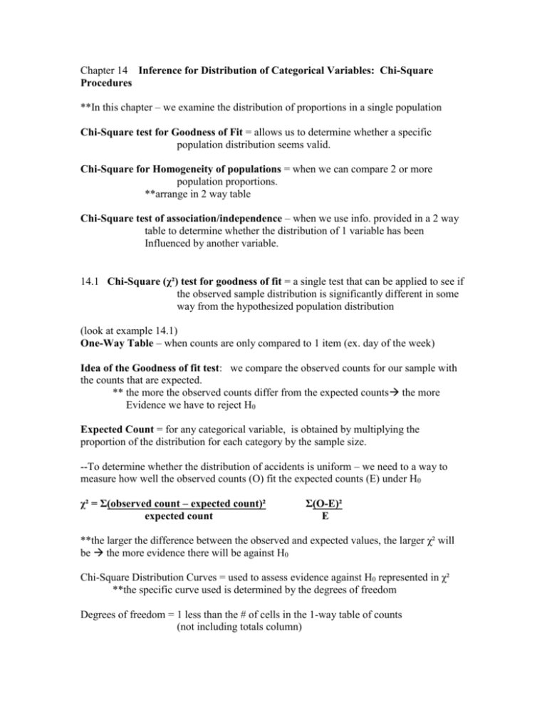
Chapter 14 Inference for Distribution of Categorical Variables: Chi-Square
Procedures
**In this chapter – we examine the distribution of proportions in a single population
Chi-Square test for Goodness of Fit = allows us to determine whether a specific
population distribution seems valid.
Chi-Square for Homogeneity of populations = when we can compare 2 or more
population proportions.
**arrange in 2 way table
Chi-Square test of association/independence – when we use info. provided in a 2 way
table to determine whether the distribution of 1 variable has been
Influenced by another variable.
14.1 Chi-Square (χ²) test for goodness of fit = a single test that can be applied to see if
the observed sample distribution is significantly different in some
way from the hypothesized population distribution
(look at example 14.1)
One-Way Table – when counts are only compared to 1 item (ex. day of the week)
Idea of the Goodness of fit test: we compare the observed counts for our sample with
the counts that are expected.
** the more the observed counts differ from the expected counts the more
Evidence we have to reject H0
Expected Count = for any categorical variable, is obtained by multiplying the
proportion of the distribution for each category by the sample size.
--To determine whether the distribution of accidents is uniform – we need to a way to
measure how well the observed counts (O) fit the expected counts (E) under H0
χ² = Σ(observed count – expected count)²
expected count
Σ(O-E)²
E
**the larger the difference between the observed and expected values, the larger χ² will
be  the more evidence there will be against H0
Chi-Square Distribution Curves = used to assess evidence against H0 represented in χ²
**the specific curve used is determined by the degrees of freedom
Degrees of freedom = 1 less than the # of cells in the 1-way table of counts
(not including totals column)
TABLE D Chi-square test statistic = a point on the horizontal axis, and the area to the
right under the curve is the p-value of the test
a) P-value = probability of observing a value of χ² at least as extreme as the one
actually observed
the larger the value of chi-square test statistic – the smaller the p value
and the more evidence you have to reject H0
 if chi-square # is not on chart, then we use .0005 and say probability of
observing a result as extreme as the one we actually observed, by
chance alone is <.05%
Test for Goodness of fit = the chi-square test applied to the hypothesis that a categorical
variable has a specified distribution
“Idea that the test assess whether the observed counts fit the hypothesized
Distribution”
A goodness of fit test = is used to help determine whether a population has a certain
hypothesized distribution, expressed as proportions of individuals
in the population falling into various outcome categories. We test:
H0: the actual population proportions are equal to the hypothesized prop.
Steps:
1. Calculate the chi-square test statistic: χ² = Σ(O-E)²
E
2. Then χ² has approximately a χ² distribution with (k-1) degrees of freedom.
For a test of H0 against the alternative:
Ha: at least 2 of the actual population proportions differ from their
hypothesized proportions
3. Conditions: may use this test with critical values from the chi-square distrib.
When all individual expected counts are at least 1, and no more than 20% of
the expected counts are less than 5 (all counts must be > 0)
Properties of Chi-Square distributions:
a) a family of distributions that take only positive values and are skewed to the
right
b) a specific chi-square distribution is specified by 1 parameter = degrees of
freedom
c) as degrees of freedom increase density curves become less skewed and
larger values become more likely
Ex,. figure 14.2
Chi-Square density curve has the following properties:
#1. Total area under chi-square curve = 1
#2. Each chi-square curve (except when df=1) begins at 0 on the horizontal axis,
increases to a peak, and then approaches the horizontal axis asymptotically from above
#3. Each chi-square curve is skewed to the right – as df increases, the curve becomes
more and more symmetrical and looks more like a normal curve
Ex. 14.3
Step 1: Hypothesis: state H0 and Ha- what are the proportions of the population- what
Falls in each category
Step 2: conditions: use chi-square goodness of fit expected counts (make sure >5)
Step 3: Calculations: use test statistic to find χ² and get p value
Step 4: Interpretation
Follow-up Analysis: in Chi-square test for goodness of fit – we test the null hypothesis
That a categorical variable has a specified distribution
Component =largest amount that contributes to χ² statistic
14.2 Inference for 2-way tables:-- use when want to compare more than 2 groups
Two-way tables: used to describe relationships between any 2 categorical variables
a) same test that compares several proportions, also tests whether the row and
column variables are related in a 2 way table
[conditional distributions vs. marginal distributions]
(review p. 293/294)
Ex. p. 850 music played = explanatory variable
Wine purchases = response variable
Problems with Multiple comparisons:
#1. How many comparisons you have to do and all the different results
 to correct: statistical methods have 2 parts:
a) an overall test to see if there are good evidence of any difference among the
parameter that we want to compare
b) a detailed follow-up analysis to decide which of the parameters differ and to
estimate how large the differences are
2-way tables: give counts for both successes and failures
** r x c table = rows x columns (not counting totals column
 shows relationship between 2 categorical variables and gives counts for all
possible combinations
Stating hypothesis: we will use the chi-square test to assess whether this observed
Association is statistically significant that is to strong to observe by
Chance
in r x c table = gives examples of separate and independent random samples
From each of c populations.
C = populations
R = values of response variables
**** allows us to compare more than 2 populations, more than 2 categories with
response or both
So H0: the distribution of the response(categorical) variable is the same in all c
populations.
Computing Expected Cell Counts – under the null hypothesis
Expected Cell Counts= row total x column total
N
Idea: 1) if we have n, independent trials and the probability of a success on each
Trial is p, we expect np successes.
2) if we draw an SRS of n individuals from a population in which the
Proportion of successes is p, we expect np successes in the sample
**expected counts need not be a whole number **
The Chi-Square test for Homogeneity of Populations
Chi-Square statistic = is a measure of how far the observed counts in a 2-way table are
from the expected counts. The formula is:
χ² = Σ(O-E)²
E
**(the sum is over all r x c in the table)
** differs from 1 way table because r =1 c=1
** must calculate the term for each cell, then sum over all cells
χ² Statistics and its P-value
χ²  is always zero or positive
a) large values of χ² are evidence against H0 because they say
that the observed counts are far from what we would expect
if H0 were true.
b) is one sided because any violation of H0 tends to produce a
large value of χ²
c) small values of χ² are not evidence against H0
**Can use same test as for goodness of fit  provided that we take separate and
independent random samples from each population
Chi-Square test for Homogenity of Population:
#1. Select independent SRS’s from each of c populations.
a) classify each individual in a sample according to a categorical response
variable with r possible values>
b) there are c different sets of proportions to be compared, one for each
population
#2. Null Hypothesis (H0) is that the distribution of the response variable is the same in all
c populations. Alternative Hypothesis (Ha) says that these c distributions are not
all the same.
#3. If H0 is true, the chi-square test statistic χ² has approximately a χ² distribution with
(r-1)(c-1) degree of freedom
#4. The p-value for the chi-square test is the area to the right of χ² under the chi-square
Density curve with (r-1)(c-1) degrees of freedom
*Chi-square (like z) becomes more accurate as the counts in the cells of the table get
Larger*
Cell counts required for the chi-square test:
You can safely use the chi-square test with critical values from the chi-square
distribution when no more than 20% of the expected counts are less than 5 and all
individual expected counts are 1 or greater. In particular, all 4 expected counts in a 2 x 2
table should be 5 or greater.
**Show on calculator
Follow-up Analysis
1) Chi-square test is overall test for comparing any # of population proportions
**the test is trying to support that we reject the null hypothesis that all
proportions are equal.
2) Size and Nature of relationship described by column row and %
3) Compare the observed and expected counts
**THIS TEST CONFIRMS THAT THERE IS A RELATIONSHIP  NOT WHAT
POPULATION OUR CONCLUSION DESCRIBES
The chi-square test and the z-test
a) if we are comparing r proportions and make the columns o f the table “successes
and failures” the counts form an r x 2 table
** can do 2 tests:
1) 2 proportion z test
2) Chi-square test with df=1
b) χ² statistic  just the square of the z statistic
c) pvalue for χ² is exactly the same as the 2 sided p value test for z
Chi-square Test of Association/ Independence
**IN example = compared 3 treatments using separate and independent samples
each group is a sample from a separate population corresponding to a separate
Treatment
Chi-Square Test of Association/Independence
***CLASSIFIES OBSERVATIONS FROM A SINGLE POPULATION
CLASSIFIED BY 2 CATEGORICAL VARIABLES ****
Null Hypothesis (H0): There is no association between 2 categorical variables
**when you have a 2-way table from a single SRS with each individual classified
according to both of 2 categorical variables.
To Do Analysis:
1. Compute the descriptive statistics (conditional distribution) that summarize the
observed relation between exclusive territory and success
(ex. categorical variables relationship is described by %)
2. The statistical test (chi-square) will tell us whether or not the difference in % can
be plausibly attributed to chance  tells us whether it is statistically significant
Computing expected cell count = can find by using the multiplication rule for
independent events:
Expected count = row total x column total (n=sample size-table total)
n
3. Perform Chi-Square test
Ex. 14.13 Inference toolbox
Distinguishing between the 2 types of Chi-Square tests for 2 way tables:
1. Examining the design of the study:
a) Test of association/independence = a single sample from a single population
(individuals are classified according to 2 categorical variables)
c) Test of homogeneity of populations – a sample from each of 2 or more
populations.
(individuals classified based on a single categorical variable)