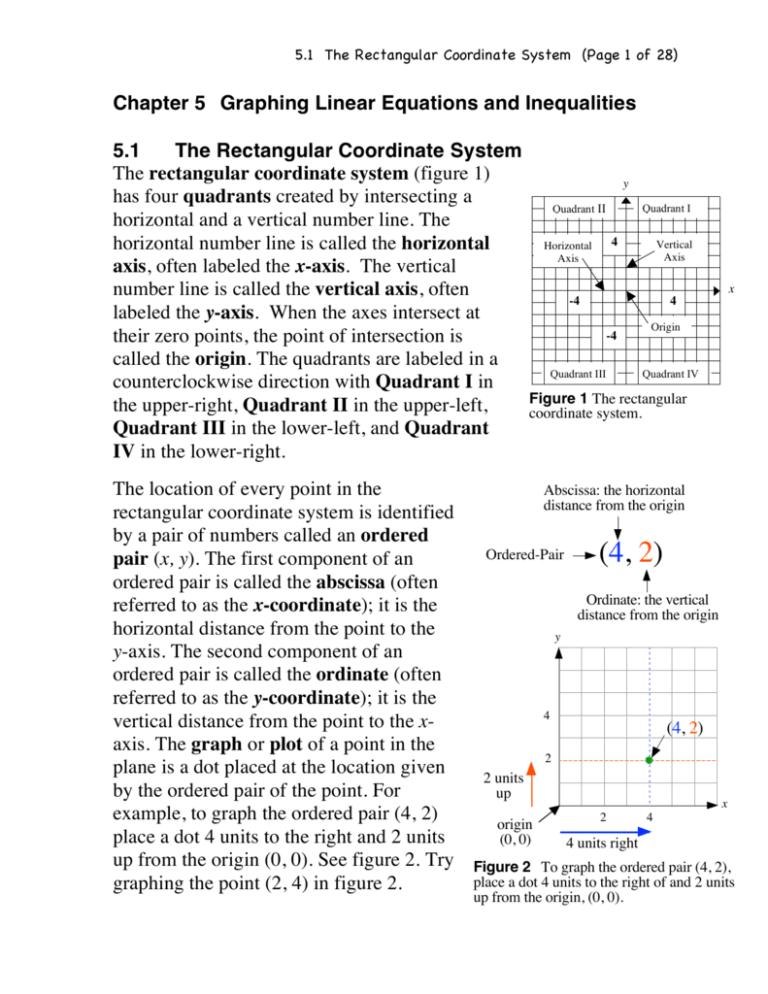
5.1 The Rectangular Coordinate System (Page 1 of 28)
Chapter 5 Graphing Linear Equations and Inequalities
5.1
The Rectangular Coordinate System
The rectangular coordinate system (figure 1)
has four quadrants created by intersecting a
horizontal and a vertical number line. The
horizontal number line is called the horizontal
axis, often labeled the x-axis. The vertical
number line is called the vertical axis, often
labeled the y-axis. When the axes intersect at
their zero points, the point of intersection is
called the origin. The quadrants are labeled in a
counterclockwise direction with Quadrant I in
the upper-right, Quadrant II in the upper-left,
Quadrant III in the lower-left, and Quadrant
IV in the lower-right.
The location of every point in the
rectangular coordinate system is identified
by a pair of numbers called an ordered
pair (x, y). The first component of an
ordered pair is called the abscissa (often
referred to as the x-coordinate); it is the
horizontal distance from the point to the
y-axis. The second component of an
ordered pair is called the ordinate (often
referred to as the y-coordinate); it is the
vertical distance from the point to the xaxis. The graph or plot of a point in the
plane is a dot placed at the location given
by the ordered pair of the point. For
example, to graph the ordered pair (4, 2)
place a dot 4 units to the right and 2 units
up from the origin (0, 0). See figure 2. Try
graphing the point (2, 4) in figure 2.
y
Quadrant II
Quadrant I
4
Horizontal
Axis
Vertical
Axis
-4
x
4
-4
Quadrant III
Origin
Quadrant IV
Figure 1 The rectangular
coordinate system.
Abscissa: the horizontal
distance from the origin
Ordered-Pair
(4, 2)
Ordinate: the vertical
distance from the origin
y
4
(4, 2)
2
2 units
up
origin
(0, 0)
x
2
4
4 units right
Figure 2 To graph the ordered pair (4, 2),
place a dot 4 units to the right of and 2 units
up from the origin, (0, 0).
5.1 The Rectangular Coordinate System (Page 2 of 28)
Example 1 Graph the following ordered pairs. Label each point and
identify the quadrant each
y
point lies in.
1.
A(2, 5) and B(5, 2)
5
2.
C(3, -6) and D(-6, 3)
-5
3.
5
x
E(4, 0) and F(0, 4)
-5
4.
G(-5, -3) and H(-3, -5)
Example 2 Identify the ordered-pair location of each point on the
graph.
A( , )
y
B( , )
A
D
C( , )
D( , )
E( , )
F( , )
4
E
G( , )
-4
B
G
-4
C
x
4
F
5.1 The Rectangular Coordinate System (Page 3 of 28)
5.1.2 Scatter Diagrams
A scatter diagram is the graph of known ordered-pair data. A
scatter diagram illustrates the visual relationship between the two
variables in the ordered pair.
Example 2
A study by the Federal Aviation Administration showed that narrow,
over-the-wing emergency exit rows slow passenger evacuation. The
table below shows the space between seats, in inches, and the
evacuation time for 35 passengers. Graph the scatter diagram for the
data.
x
Space
Between
Seats
(inches)
y
Evacuation
Time
(seconds)
6
10
13
15
20
44
43
38
36
37
Evacuation Time (seconds)
y
45
40
35
x
30
0
5
10
15
20
25
Space Between Seats (inches)
5.1.3 Average Rate of Change
Given two ordered-pairs (x1 , y1 ) and (x 2 , y2 ) the average rate of
change (ARC) of y with respect to x is given by
ARC =
change in y second y value - first y value y2 ! y1
=
=
change in x second x value - first x value x 2 ! x1
Example 3
From the data in example 3, find the average rate of change (ARC)
using the points (6, 44) and (20, 37). Analyze the units of the ARC to
interpret your results.
5.2 Graphs of Linear Equations (Page 4 of 28)
5.2 Graphs of Linear Equations (Straight Lines)
5.2.1 Linear Equations in Two Variables in the form
y = mx + b
A linear equation in two variables is any equation whose graph
forms a straight line. One form of a linear equation in two variables is
y = mx + b , where x and y are the variables, m is the [constant]
coefficient of x, and b is also a constant. A second form will be
discussed in the next section.
Example 1 For each equation, identify the constants m and b.
Equation, y = mx + b
y = 3x + 4
y = !x ! 7
y = !3
y = !5x
2
y= ! x+3
3
m
3
b
4
Solution to a Linear Equation in Two Variables
A solution to a linear equation in two variables is an ordered pair
of numbers (x, y) that [when substituted for the variables] makes the
equation true.
Example 2
Is (3, -5) a solution to y = !3x + 4 ?
Example 3
" 2
%
Is $ ! , ! 2 ' a solution to y = !3x + 4 ?
# 3
&
5.2 Graphs of Linear Equations (Page 5 of 28)
5.2.2 Graphs of Linear Equations in the form y = mx + b
Equations with two variables have an infinite number of ordered-pair
solutions. The graph of an equation in two variables is a drawing
of all the ordered-pair solutions to the equation. The graph of every
linear equation in two variables (i.e. y = mx + b ) forms a straight line.
Graphing Linear Equations by Plotting Three Points
To graph a linear equation in the form y = mx + b :
1. Pick three values for x.
2. For each x chosen in step 1, use the given equation, y = mx + b , to
compute the three corresponding values of y.
3. Plot the three ordered pairs and use a ruler to draw a straight line
through the points. Draw the line through the entire grid and draw
arrowheads at each end of the line to show that the line continues
indefinitely.
Example 5
y
Graph y = 2x ! 3 by
finding three solutions.
5
-5
5
-5
x
5.2 Graphs of Linear Equations (Page 6 of 28)
y
Example 6
Graph y = !3x + 2 by
finding three solutions.
5
-5
5
x
5
x
5
x
-5
Example 7
y
2
Graph y = x ! 4 by
3
finding three solutions.
5
-5
-5
Example 8
y
1
Graph y = ! x + 3 by
2
finding three solutions.
5
-5
-5
5.2 Graphs of Linear Equations (Page 7 of 28)
5.2.3
Graphs of Equations in the form Ax + By = C
Steps to graph a linear equation in the form Ax + By = C
To graph a linear equation in the form Ax + By = C :
1. Solve Ax + By = C for y. That is, isolate y to get the equation in
the form y = mx + b .
2. Graph by plotting three points.
i. Pick three values for x.
ii. For each x chosen in step i, use the equation from step i
( y = mx + b ) to compute the three corresponding values of y.
iii. Plot the three ordered pairs and use a ruler to draw a line
through the points. Draw the line through the entire grid and
draw arrowheads at each end of the line to show that the line
continues indefinitely.
Example 10 Graph 2x + 3y = 6 by finding three solutions.
1.
Solve the equation for y.
y
2.
Compute three points and graph.
5
Pick x
Compute y =
Plot (x, y)
x=
-5
5
x=
x=
-5
3. Write the ordered-pair where the
graph intersects the x-axis.
4. Write the ordered-pair where the graph intersects the y-axis.
x
5.2 Graphs of Linear Equations (Page 8 of 28)
Example 11 Graph 2x ! 5y = 10 by finding three solutions.
1.
Solve the equation for y.
y
2.
Plot three points and graph.
Pick x
Compute y =
5
Plot (x, y)
x=
-5
5
x=
-5
x=
3. The x-intercept in a graph is the ordered-pair (x, y) location
where the graph intersects the x-axis.
Write the x-intercept in the graph of 2x ! 5y = 10 .
What is the value of the y-component of the x-intercept?
4. The y-intercept in a graph is the ordered-pair (x, y) location
where the graph intersects the y-axis.
Write the y-intercept in the graph of 2x ! 5y = 10 .
What is the value of the x-component of the y-intercept?
x
5.2 Graphs of Linear Equations (Page 9 of 28)
5.2.4
Graph lines using the x- and y-Intercepts
Intercepts of a Curve (Graph)
The x-intercept of a graph is the point (ordered pair location) where
the graph intersects the x-axis. The y-intercept of a graph is the
ordered pair location where the graph intersects the y-axis.
Example 5
a. Identify the intercepts of each curve.
A
4
Curve x-intercept y-intercept
A
B
C
(
(
(
,
,
,
)
)
)
(
(
(
,
,
,
)
)
)
y
-4
4
-4
b. What is the y value of all x-intercepts?
c.
B
C
What is the x value of all y-intercepts?
Finding intercepts when given an equation.
1. All x-intercepts are in the form (a, 0), where a is a constant
[number]. To find the x-intercept, set y = 0 and solve for x.
2. All y-intercepts are in the form (0, a), where a is a constant. To
find the y-intercept, set x = 0 and solve for y.
x
5.2 Graphs of Linear Equations (Page 10 of 28)
Example 12 Find the x- and y-intercepts in the graph of
5x + 4 y = 20 . Then graph the line.
Solution
An x-intercept is in the form (?, 0). Thus, set y = 0 and find the
corresponding value of x.
Set y = 0
An x-intercept
is in the form (? , 0)
The x-intercept
(4, 0)
5x + 4y = 20
5x + 4(0) = 20
5x
= 20
is
x=4
Solve for x
A y-intercept is in the form (0, ?). Thus, set x = 0 and find the
corresponding value of y.
Set x = 0
5x + 4y = 20
A y-intercept
5(0) + 4y = 20
is in the form (0 , ?)
4y = 20
The y-intercept is
y=5
Solve for y
(0, 5)
y
Thus, the x-intercept is (4, 0) and the yintercept is (0, 5). Now, graph the line
using the intercepts.
5
-5
5
-5
x
5.2 Graphs of Linear Equations (Page 11 of 28)
Example 13 Find the x- and y-intercepts of !3x + 7y = 21 and
graph the line.
y
5
-5
5
x
-5
Example 15 Find the x- and y-intercepts of 3x ! 4 y = 12 and graph
the line.
y
5
-5
5
-5
x
5.2 Graphs of Linear Equations (Page 12 of 28)
Mentally finding an x-intercept
Recall, an x-intercept is in the form (___, 0). So, to find the xintercept set y = 0 and solve for the x-coordinate. Then write the
intercept as an ordered-pair. Since setting y = 0 makes the term
containing y disappear, you can simply cover the “y-term” and
mentally solve for x. In the following illustration, the shaded-out
parts indicate the computations done mentally:
Conventional
method of finding
the x-intercept
Mentally find
the x-intercept
!4x ! y = 8
!4x ! 0 = 8
!4x
=8
!4x ! y = 8
8
x
=
x
= !2
Since y = 0, the term
containing y disappears.
So, just put your finger
over the y-term and
mentally solve –4x = 8
to get x = -2.
x
=
x
= !2
x ! int . is (!2, 0)
8
!4
!4
Thus the x-intercept is (-2, 0). Similarly, covering the x-term will
allow you to mentally find that the y-intercept is (0, -8).
Example 16
Find the x- and y-intercepts in the graph of each equation.
Equation
x-intercept
A B C
Ax + By = C
(a, 0)
3x + 4 y = 12
2x ! 5y = 10
x ! 2y = !6
x ! 2y = !9
!x + 3y = !2
3
4 12
(4, 0)
y-intercept
(0, b)
(0, 3)
5.2 Graphs of Linear Equations (Page 13 of 28)
Equations & Graphs of Horizontal and Vertical Lines
y
Horizontal Lines
All horizontal lines have the
equation y = b , where b is a constant.
The y-intercept in the graph of y = b
is (0, b).
y=b
(0, b)
x
y
Vertical Lines
All vertical lines have the equation
x = a , where a is a constant. The xintercept in the graph of x = a is
(a, 0).
x=a
x
(a, 0)
Example 18 Graph each equation. Label each graph.
a.
x = !5
b.
y=7
c.
x=3
d.
y = !1
y
5
-5
e.
f.
What is the equation of line lying on
the x-axis?
What is the equation of the line lying
on the y-axis?
5
-5
x
5.3: Slope of a Line (Page 14 of 28)
5.3.1 Slope of a Line
The measure of a line’s slant is called the slope of the line, denoted
m. The slope of a non-vertical line containing the two points
P1 (x1 , y1 ) and P2 (x 2 , y2 ) is given by
rise y2 ! y1 "y
m=
=
= .
run x 2 ! x1 "x
y
read “change in y “
read “change in x“
y
P2 (x 2 , y 2 )
P2
y2
rise
P1
rise = y 2 ! y1
P1 (x1, y1 )
y1
run
run = x 2 ! x1
x
x
x2
x1
Figure 1 Slope of a line, m =
rise y 2 ! y1
=
run x 2 ! x1
Example 1
a. Graph the line containing the two
points (!2, 4) and (8, !1) . Then
compute the slope of the line.
y
5
-5
b. Pick two other points on the line in
part a and compute the slope of the
line using those two points.
5
-5
c. A line that falls from left to right is called a decreasing line.
Decreasing lines have a slope that is [positive negative].
circle
one
x
5.3: Slope of a Line (Page 15 of 28)
Example 2
a. Graph the line containing the two
points (!5, ! 5) and (7, 3) . Then
compute the slope of the line.
y
5
-5
b. A line that rises from left to right is
called an increasing line. Increasing
lines have a slope that is [positive
negative].
5
x
5
x
-5
Example 3
a. Graph the line containing the two
points (6, 4) and (6,1) . Then compute
the slope of the line.
y
5
b. Vertical lines have a slope that is
[positive negative zero undefined].
-5
-5
c. List three other ordered-pairs on the
line.
d. What is the equation of the line?
5.3: Slope of a Line (Page 16 of 28)
y
Example 4
a. Graph the line containing the two
points (!7, ! 5) and (1, ! 5) . Then
compute the slope of the line.
5
-5
b. Horizontal lines have a slope that is
[positive negative zero undefined].
5
x
-5
c. List three other ordered-pairs on the
line.
d. What is the equation of the line?
Example 5
a. Graph the line containing the two points
(6, 3) and (!2, 7) . Then compute the
slope of the line.
b. Graph the line containing the two points
(6, !1) and (2,1) . Then compute the
slope of the line.
c. What can be said about the two lines
from parts a and b?
y
5
-5
5
-5
x
5.3: Slope of a Line (Page 17 of 28)
5.3.2
Slopes of Parallel and Perpendicular Lines
Slopes of Parallel lines
Two non-vertical lines are parallel if and only if their slopes are
equal. The preceding statement is equivalent to the following three:
1. If two non-vertical lines are parallel, then their slopes are equal.
2. If two non-vertical lines have equal slopes, then they are parallel.
3. All vertical lines are parallel.
Slopes of Perpendicular lines
Two lines are perpendicular if and only if their slopes are opposite
reciprocals of each other. That is, if two lines l1 and l2 have slopes
m1 and m 2 , respectively, then the preceding statement is equivalent to
the following three:
1
1. If l1 is perpendicular to l2 , then m1 = ! .
m2
1
2. If m1 = ! , then l1 is perpendicular to l2 .
m2
3. Every horizontal line is perpendicular to every vertical line.
Example 6
For each slope given,
fill-in the table
with the slope of every
line parallel to and
perpendicular to a line
with the given slope.
Slope
2
3
!4
!
3
8
0
undefined
Slope of any
parallel line
Slope of any
perpendicular
line
5.3: Slope of a Line (Page 18 of 28)
Example 7
a. Graph the line containing the two
points (6, 3) and (!2, 7) . Then
compute the slope of the line.
y
5
-5
b. Graph the line containing the two
points (!2, ! 3) and (3, 7) . Then
compute the slope of the line.
c. What can be said about the two
lines from parts a and b?
5
-5
x
5.3: Slope of a Line (Page 19 of 28)
5.3.2 Graph a line using the slope and y-intercept
Slope-Intercept Form of a Straight Line
The Slope-Intercept Form of a Straight Line is given by y = mx + b ,
where the slope of the line is m and the y-intercept is (0, b).
To find the y-intercept,
set x = 0
Example 1 Identify the slope and y-intercept in the graph of each
equation.
Equation, y = mx + b
3
y = ! x +1
4
Slope = m
y-intercept, (0, b)
y = 2x ! 4
x
y = +5
2
y = !x
y=2
Example 2 Graph y = 2x ! 3 using the
slope and y-intercept.
i. Identify the slope and y-intercept.
y
5
ii. Plot the y-intercept.
rise
, to generate
run
other points on the line.
iii. Use the slope, m =
-5
5
-5
x
5.3: Slope of a Line (Page 20 of 28)
y
Example 3 Use the slope and yintercept to graph
2
y = ! x +1.
3
5
-5
5
x
5
x
5
x
-5
y
Example 4 Use the slope and yintercept to graph
1
y = ! x ! 2.
4
5
-5
-5
y
Example 5 Use the slope and yintercept to graph
y = 3x + 5 .
5
-5
-5
5.4: Finding the Equation of a Line (Page 21 of 28)
5.4.1 Finding the Equation of a Straight Line Using the
Slope-Intercept form of a line ( y = mx + b )
When asked to find the equation of a line using the slope-intercept
form ( y = mx + b ) of the line, the goal is to find the constants m and b
(x and y remain as variables).
Steps to find the equation of a straight line
using the slope-intercept form of a line ( y = mx + b )
1. Substitute the given values for x, y and m into y = mx + b and
solve for the value of b.
2. Keep x and y as variables and substitute the now known values
for m and b into the equation y = mx + b .
Example 1
Find the equation of the line that has slope 3 and
passes through the point (0, 2).
Set m = _____, x = _____, and y = _____ in the equation
y = mx + b , and solve for b. Then write the equation in the form
y = mx + b .
Example 2 Find the equation of the line that has slope -1/2 and
passes through the point (-2, 4).
Set m = _____, x = _____, and y = _____ in the equation
y = mx + b , and solve for b. Then write the equation in the form
y = mx + b .
5.4: Finding the Equation of a Line (Page 22 of 28)
Example 3 Find the equation of the line that has slope 2/3 and
passes through the point (3, -3).
Example 4 Find the equation of the line that has slope –3/2 and
passes through the point (4, - 2).
5.4: Finding the Equation of a Line (Page 23 of 28)
5.4.2
Finding the Equation of a line using the Point-Slope
formula, y ! y1 = m(x ! x1 )
Point-Slope Formula for a Line
The point-slope formula for a line is y ! y1 = m(x ! x1 ) , where the
line has slope m and passes through the point whose coordinates are
(x1 , y1 ).
Example 1 Use the point-slope formula to find the equation of the
line that that passes through the point (!2, !1) and has
slope 3/2.
5.4.3
Finding the Equation of a line given two points on
the line.
Example 2
Find the equation of the line that passes through the
points (-4, -5) and (8, 4).
5.4: Finding the Equation of a Line (Page 24 of 28)
Example 3
Find the equation of the line that passes through the
points (-3, -9) and (1, -1).
y
Example 4
a.
Find the equation of line 1.
4
-4
4
-4
b.
Find the equation of line 2.
Skip section 5.5
line 1
line 2
x
5.6: Graphing Linear Inequalities (Page 25 of 28)
5.6 Graphing Linear Inequalities in Two Variables
Linear Inequality in two Variables
A linear inequality in two variables is two expressions separated by
one of the inequality symbols (<, >, !, ") .
Example 1
y
Graph y = x ! 2
5
-5
5
-5
Note
The graph of y = x ! 2 separates the coordinate plane into
three disjoint sets of points:
The set of points y = x ! 2 , which lie on the
line.
1.
On the Line:
2.
Above the Line: The set of points y > x ! 2 , which lie
“above” the line. The region above the line
is called the upper half-plane.
3.
Below the Line: The set of points y < x ! 2 , which lie
“below” the line. The region below the line
is called the lower half-plane.
x
5.6: Graphing Linear Inequalities (Page 26 of 28)
Steps to Graph an Inequality
1. Solve the inequality for y (isolate y).
2. Graph the line y = mx + b as a solid or dashed line as follows:
a. Draw a solid line if the inequality from step 1 is in the form
y ! mx + b or y ! mx + b . A solid line indicates the line is part
of the solution set.
b. Draw a dashed line if the inequality from step 1 is in the form
y > mx + b or y < mx + b . A dashed line indicates the line is
just a boundary and is not part of the solution set.
3. Shade-in the upper half-plane or the lower half-plane as follows:
a. Shade-in the region above the line if the inequality from step 1
is in the form y > mx + b or y ! mx + b .
b. Shade-in the region below the line if the inequality from step 1
is in the form y < mx + b or y ! mx + b .
Example 2
Graph the solution set to 2x ! 3y " 6 .
Example 3
Graph the solution set to 2x ! 3y > 6 .
y
y
5
-5
5
5
-5
x
-5
5
-5
x
5.6: Graphing Linear Inequalities (Page 27 of 28)
Example 4
Graph the solution set to 3x + y > !2 .
y
5
-5
5
x
5
x
-5
Example 5
Graph the solution set to x ! 3y " 2 .
y
5
-5
-5
5.6: Graphing Linear Inequalities (Page 28 of 28)
Graph the solution set to (a) y > 3 , and (b) x ! 4 .
Example 6
a. y > 3 .
b.
x!4
y
y
4
4
-4
x
4
-4
-4
Example 7
x
4
-4
Write the inequality for each graph shown.
a.
b.
y
y
4
4
-4
4
-4
x
-4
4
-4
x