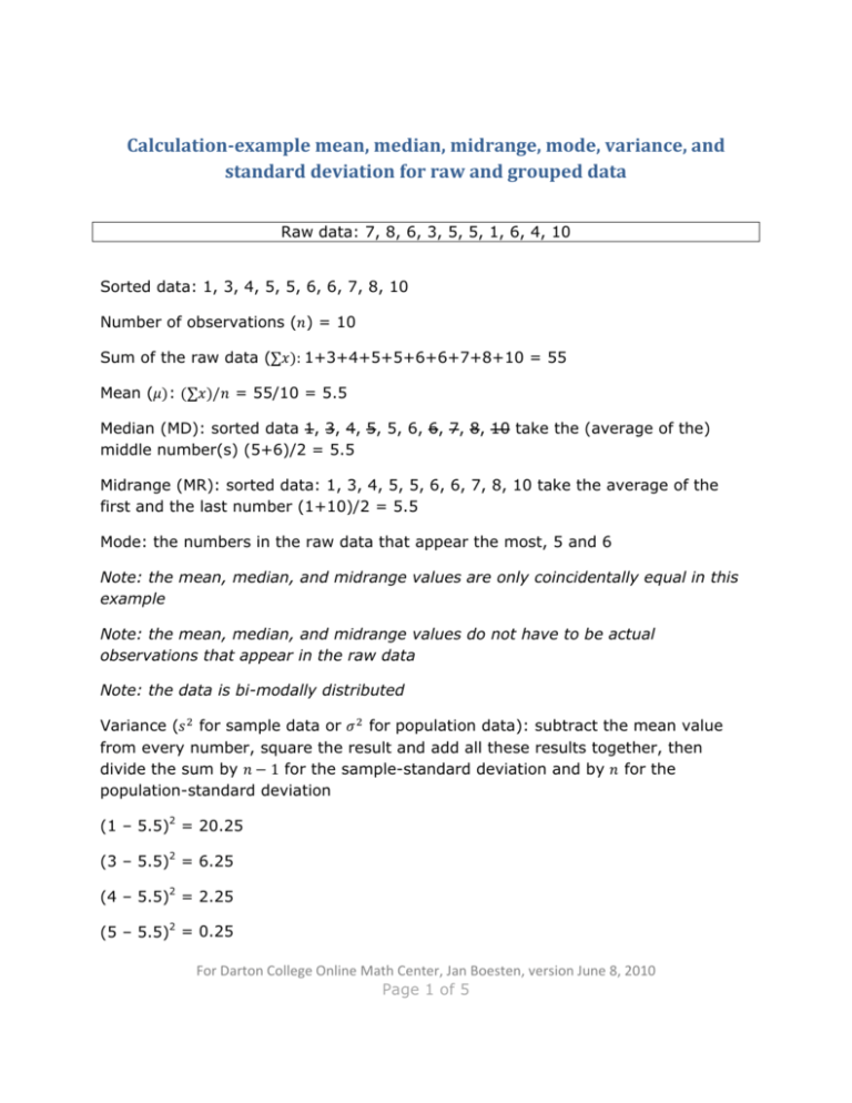
Calculation­example mean, median, midrange, mode, variance, and standard deviation for raw and grouped data Raw data: 7, 8, 6, 3, 5, 5, 1, 6, 4, 10
Sorted data: 1, 3, 4, 5, 5, 6, 6, 7, 8, 10
Number of observations ( ) = 10
Sum of the raw data (∑ : 1+3+4+5+5+6+6+7+8+10 = 55
Mean ( : ∑ / = 55/10 = 5.5
Median (MD): sorted data 1, 3, 4, 5, 5, 6, 6, 7, 8, 10 take the (average of the)
middle number(s) (5+6)/2 = 5.5
Midrange (MR): sorted data: 1, 3, 4, 5, 5, 6, 6, 7, 8, 10 take the average of the
first and the last number (1+10)/2 = 5.5
Mode: the numbers in the raw data that appear the most, 5 and 6
Note: the mean, median, and midrange values are only coincidentally equal in this
example
Note: the mean, median, and midrange values do not have to be actual
observations that appear in the raw data
Note: the data is bi-modally distributed
Variance ( for sample data or
for population data): subtract the mean value
from every number, square the result and add all these results together, then
divide the sum by
1 for the sample-standard deviation and by for the
population-standard deviation
(1 – 5.5)2 = 20.25
(3 – 5.5)2 = 6.25
(4 – 5.5)2 = 2.25
(5 – 5.5)2 = 0.25
For Darton College Online Math Center, Jan Boesten, version June 8, 2010 Page 1 of 5
(5 – 5.5)2 = 0.25
(6 – 5.5)2 = 0.25
(6 – 5.5)2 = 0.25
(7 – 5.5)2 = 2.25
(8 – 5.5)2 = 6.25
(10 – 5.5)2 = 20.25
20.25+6.25+2.25+0.25+0.25+0.25+0.25+2.25+6.25+20.25 = 58.5
= 58.5 / (10-1) = 6.5 and
= 58.5 / 10 = 5.85
Standard deviation ( for sample data or
root of the variance
= √6.5 = 2.55 and
for population data): take the square
= √5.85 = 2.42
Create a histogram with four classes and calculate the statistics/parameters (mean, median, and mode) from the grouped sample/population data Range of values: sorted data 1, 3, 4, 5, 5, 6, 6, 7, 8, 10 subtract first number from
last number 10-1 = 9
Class-width: divide range of values by number of classes and round up to the same
number of decimals as the raw data 9/4 = 2.25 rounded to 3
Determine the first and second class to establish a pattern:
Class 1: first number is 1; class-width is three so in class the numbers 1, 2, and 3
Class 2: first number is 4; class-width is three so in class the numbers 4, 5, and 6
Pattern:
Class 1: 1 – 3
Class 2: 4 – 6
Class 3: 7 – 9
Class 4: 10 – 12
For Darton College Online Math Center, Jan Boesten, version June 8, 2010 Page 2 of 5
Note: the pattern for the lower class-limits 1, 4, 7, and 10 (add three to previous
number); pattern for upper class-limits 3, 6, 9, and 12 (add three to previous
number)
Class-limits: class 1: 1 – 3, class 2: 4- 6, class 3: 7 – 9, class 4: 10 – 12
Class-boundaries: class 1: 0.5 – 3.5, class 2: 3.5- 6.5, class 3: 6.5 – 9.5, class 4:
9.5 – 12.5
For classes with decimal class-limits:
Class-limits: class 1: 0.5 – 2.5, class 2: 2.6- 4.6, class 3: 4.7 – 6.7, class 4: 6.8 –
8.8
Class-boundaries: class 1: 0.45 – 2.55, class 2: 2.55- 4.65, class 3: 4.65 – 6.75,
class 4: 6.75 – 8.85
Note: the class-limits should have the same decimal place value as the data, but
the class-boundaries should have one additional place value and end in a five
Note: the class-width can be found by subtracting the lower boundary from the
upper boundary for any given class; do NOT subtract the lower limit from the upper
limit of a single class since that will result in an incorrect answer
Classes and their frequencies:
Sorted data: 1, 3, 4, 5, 5, 6, 6, 7, 8, 10
Class
Class
Class
Class
Class
1:
2:
3:
4:
0.5
3.5
6.5
9.5
–
–
–
–
3.5
6.5
9.5
12.5
Frequency (
2
5
2
1
Cumulative frequency (∑
2
7
9
10
Note: the first column may start at 0.5 instead of 0; the histogram below starts its
first column at 0
For Darton College Online Math Center, Jan Boesten, version June 8, 2010 Page 3 of 5
Histogram:
Title
6
5
4
3
frequency
2
1
0
Class 1
Class 2
Class 3
Class 4
: take the average of the sum of the lower boundary and the
Class midpoint (
upper boundary (or the average of the sum of the lower limit and the upper limit)
(0.5+3.5)/2 = 2 (or (1+3)/2 = 2); (3.5+6.5)/2 = 5 (or (4+6)/2 = 5); (6.5+9.5)/2
= 8 (or (7+9)/2 = 8); (9.5+12.5)/2 = 11 (or (10+12)/2 = 11)
Class midpoints (
: 2, 5, 8, and 11
Note: it is preferable that the class-width be an odd number. This ensures that the
midpoint of each class has the same place value as the data
Mean ( : multiply the class midpoint with the corresponding class frequency and
sum the results for all classes, then divide the result by the sum of the frequencies
Class midpoints times class frequencies: 2*2 = 4, 5*5 = 25, 8*2 = 16, and 11*1 =
11
Sum the results: 4+25+16+11 = 56
Summation of all frequencies: 2+5+2+1 = 10
For Darton College Online Math Center, Jan Boesten, version June 8, 2010 Page 4 of 5
Mean ( ): 56/10 = 5.6
Median (MD): observe the cumulative frequencies for the data (previous page) and
note that with 10 numbers, the median numbers are the fifth and sixth number in
the sorted data; the fifth and sixth numbers are in Class 2
Calculate the Median (MD) with the following formula:
MD =
L = lower limit of the class containing the median value(s)
n = cumulative frequency
CF = the cumulative frequency of the class(es) preceding the median class
f = the frequency of the class containing the median value(s)
i = class-width of the median class
Then:
L=4
n = 10
CF = 2
f=5
i=3
MD = 4
3=4
3 = 5.8
Mode: the class(es) with the highest frequency, Class 2
Note: when raw data is grouped and statistics/parameters are calculated from the
classes, accuracy gets lost.
For Darton College Online Math Center, Jan Boesten, version June 8, 2010 Page 5 of 5