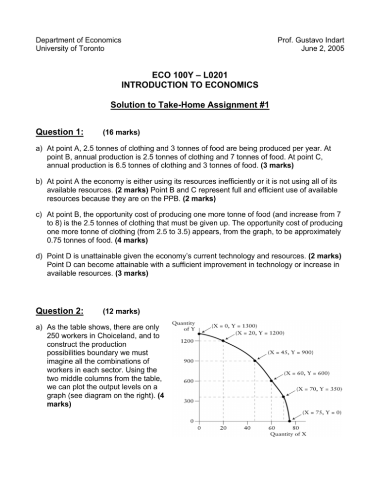
Department of Economics
University of Toronto
Prof. Gustavo Indart
June 2, 2005
ECO 100Y – L0201
INTRODUCTION TO ECONOMICS
Solution to Take-Home Assignment #1
Question 1:
(16 marks)
a) At point A, 2.5 tonnes of clothing and 3 tonnes of food are being produced per year. At
point B, annual production is 2.5 tonnes of clothing and 7 tonnes of food. At point C,
annual production is 6.5 tonnes of clothing and 3 tonnes of food. (3 marks)
b) At point A the economy is either using its resources inefficiently or it is not using all of its
available resources. (2 marks) Point B and C represent full and efficient use of available
resources because they are on the PPB. (2 marks)
c) At point B, the opportunity cost of producing one more tonne of food (and increase from 7
to 8) is the 2.5 tonnes of clothing that must be given up. The opportunity cost of producing
one more tonne of clothing (from 2.5 to 3.5) appears, from the graph, to be approximately
0.75 tonnes of food. (4 marks)
d) Point D is unattainable given the economy’s current technology and resources. (2 marks)
Point D can become attainable with a sufficient improvement in technology or increase in
available resources. (3 marks)
Question 2:
(12 marks)
a) As the table shows, there are only
250 workers in Choiceland, and to
construct the production
possibilities boundary we must
imagine all the combinations of
workers in each sector. Using the
two middle columns from the table,
we can plot the output levels on a
graph (see diagram on the right). (4
marks)
2
b) If the economy is already producing 60 units of X and 600 units of Y, then 10 extra units of
X can only be produced by reducing the production of Y by 250 units. (2 marks) The
opportunity cost of 10 units of X is therefore 250 units of Y (or 25 units of Y per unit of X).
If the economy is already producing 70 units of X, the opportunity cost of producing an
additional 5 units of X is the forgone 350 units of Y (or 70 units of Y per unit of X). Thus,
we see that the opportunity cost of X rises when more of X is already being produced. (3
marks)
c) If any given amount of labour can now produce 10 percent more of good Y, then the PPB
shifts up in a particular way. Specifically, the Y values increases by 10 percent for any
given X value, as shown below. (3 marks)
Question 3:
(12 marks)
a) You can catch 3 rabbits or 6 fish in one day’s work. Thus, your opportunity cost for an
additional rabbit is 2 fish. (2 marks) For your friend, the opportunity cost of an additional
rabbit is 4 fish. (2 marks)
Note: This question has not been phrased properly, and thus there is not a unique correct
answer. The assumption that “one fish represents the same amount of food as one rabbit”
doesn’t make sense and affects the intention of the question. The correct assumption should
have been that “three fish represent the same amount of food as one rabbit.”
b) To allocate tasks in the output-maximizing way, each person should do the task for which
they have the lower opportunity cost. You have the lower opportunity cost of catching
rabbits. Your friend has the lower opportunity cost for catching fish (0.25 of a rabbit for
your friend as compared to 0.5 of a rabbit for you). So to maximize output you should
3
focus on catching rabbits and your friend should focus on catching fish. In this way, the
total amount of food would be 17, i.e., the equivalent of 3 rabbits and 8 fish. (4 marks)
[Note that answering that both should catch fish (i.e., 14 fish) was considered a correct
answer given the wrong assumption stated in the question.]
c) If instead you catch rabbits and your friend catches fish, there would be a total output
(after two days’ work) of 6 rabbits and 16 fish. [Note that answering 28 fish was accepted
as a correct answer.] (2 marks) The reverse allocation would yield only 4 rabbits and 12
fish, which is clearly inferior. [Note that the reverse allocation being 5 rabbits was also
accepted as a correct answer.] (2 marks)
Question 4:
(10 marks)
a) Using Calgary as the “base university” means that we choose $6.25 as the base price.
This means dividing all prices by $6.25 and then multiplying by 100. In this way, we will
determine, in percentage terms, how prices at other universities differ from Calgary prices.
The index values are as follows: (4 marks)
University
Price
per
pizza
Index of pizza prices
Dalhousie
Laval
McGill
Queen’s
Waterloo
Manitoba
Saskatchewan
Calgary
UBC
Victoria
$6.50
5.95
6.00
8.00
7.50
5.50
5.75
6.25
7.25
7.00
(6.50/6.25)×100 = 104
(5.95/6.25)×100 = 95.2
(6.00/6.25)×100 = 96
(8.00/6.25)×100 = 128
(7.50/6.25)×100 = 120
(5.50/6.25)×100 = 88
(5.75/6.25)×100 = 92
(6.25/6.25)×100 = 100
(7.25/6.25)×100 = 116
(7.00/6.25)×100 = 112
b) The university with the most expensive pizza is Queen’s, at $8.00 per pizza. The index
value for Queen’s is 128, indicating that pizza there is 28 percent more expensive than at
Calgary. (2 marks)
c) The university with the least expensive pizza is Manitoba, at $5.50 per pizza. The index
value for Manitoba is 88, indicating that the price of pizza there is only 88 percent of the
price at Calgary. It is therefore 12 percent cheaper than at Calgary. (2 marks)
d) These are cross-sectional data. The variable is the price of pizza, collected at different
places at a given point in time (March 1, 2004). If the data had been the prices of pizza at
a single university at various points in time, they would be time-series data. (2 marks)
4
Question 5:
(12 marks)
a) The simple average of the three regional unemployment rate is equal to (5.5 + 7.2 +
12.5)/3 = 8.4. (2 marks) Is 8.4% the “right” unemployment rate for the country as a
whole? The answer is no because this simple, unweighted (or, more correctly, equally
weighted) average does not account for the fact that the Centre is much larger in terms of
the labour force than either the West or East, and thus should be given more weight than
the other two regions. (2 marks)
b) To solve this problem, we construct a weighted average unemployment rate. We do so by
constructing a weight for each region equal to that region’s share in the total labour force.
These weights are:
West:
weight = 5.3/17.2 = 0.308
Centre: weight = 8.4/17.2 = 0.488
East:
weight = 3.5/17.2 = 0.203
These weights should sum exactly to 1.0, but due to rounding they do not quite do so.
Using these weights, we now construct the average unemployment rate as the weighted
sum of the three regional unemployment rates.
Canadian unemployment rate = (.308 × 5.5) + (.488 × 7.2) + (.203 × 12.5) = 7.75 (6
marks)
This is a better measure of the Canadian unemployment rate because it correctly weights
each region’s influence in the national total. Keep in mind, however, that for many
situations the relevant unemployment rate for an individual or a firm may be the more
local one rather than the national average. (2 marks)
Question 6: (20 marks)
a) The demand curve is: QD = 100 – 3p. This is a straight-line demand curve with a slope of –
1/3. The horizontal intercept (p=0) is QD=100. The vertical intercept (QD=0) is p=33.33. The
supply curve is: QS = 10 + 2p. This is a straight-line supply curve with a slope of ½. When
p=0, QS = 10. Both curves are plotted below. (2 marks)
5
b) Equilibrium requires QD = QS. This equality defines the equilibrium price, p*. (2 marks)
c) Imposing QD = QS, we have 100 - 3p = 10 + 2p. Solving for p we get 90 = 5p or p = 18. This
is what we call p*, the market-clearing price. (2 marks)
d) Substituting p* = 18 into the demand function we get Q* = 100 - 3(18) = 46. If we substitute
p* instead into the supply function we get Q* = 10 + 2(18) = 46. (Of course, since the
demand and supply curves intersect at p* = 18, it follows that Q* must be the same whether
we use the demand curve or the supply curve.) (2 marks)
e) Now there is an increase in demand. The new demand function is QD = 180 - 3p.
Equilibrium requires QD = QS which means 180 – 3p = 10 + 2p. The solution for p* is
therefore 5p* = 170 or p* = 34. Substituting p* back into the demand curve we get Q* =
180 - 3(34) or Q* = 78. (4 marks) The law of demand says that an increase in demand
leads to a rise in both the equilibrium price and the equilibrium quantity. Both predictions
are correct. (2 marks)
f) Now with the new demand curve in place there is an increase in supply. The new supply
curve is QS = 90 + 2p. Equilibrium requires 180 – 3p = 90 + 2p. This gives p* = 18.
Substituting p* back into the demand curve leads to Q* = 180 – 3(18) or Q* = 126. (4
marks) The law of supply says that an increase in supply leads to a fall in price and a rise
in quantity. Both predictions are correct. (2 marks)
Question 7: (18 marks)
a) The diagram below shows the relevant information and assumes that both demand and
supply curves are linear. Point E is the initial equilibrium. (3 marks)
b) An increase in price from $1.00 to $1.50 per can leads to a reduction in quantity
demanded from 4200 to 3000 cans per month. Thus the own-price elasticity of demand is:
6
η = (1200/3600)/(0.50/1.25) = (1/3)/(2/5) = 5/6 (4 marks)
This is relatively inelastic demand. (1 marks)
c) An increase in price from $1.00 per can to $1.50 per can leads to an increase in quantity
supplied from 4200 to 4500 cans per month. Thus the own-price elasticity of supply is:
ηS = (300/4350)/(0.50/1.25) = 0.0689/0.4 = 0.17 (4 marks)
This is relatively inelastic supply. (1 marks)
d) The availability of substitutes is the key factor affecting elasticity. How willing and able are
consumers to substitute to competing products, such as frozen grape juice, apple juice,
milk, or soft drinks? (2 marks) Another less relevant factor would be the weight of
expenditure on orange juice in total expenditure for the average consumer. (1 mark)
e) The ability of producers to substitute toward the production of other goods is the key
factor affecting supply elasticity. Can their equipment be used for other purposes? Can
their management skills be easily shifted? (2 marks)