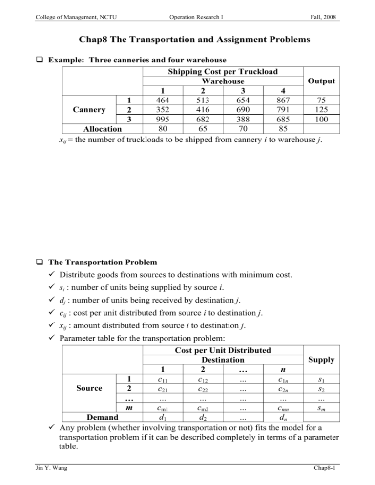
College of Management, NCTU
Operation Research I
Fall, 2008
Chap8 The Transportation and Assignment Problems
‰ Example: Three canneries and four warehouse
Shipping Cost per Truckload
Output
Warehouse
1
2
3
4
464
513
654
867
75
1
Cannery
352
416
690
791
125
2
995
682
388
685
100
3
80
65
70
85
Allocation
xij = the number of truckloads to be shipped from cannery i to warehouse j.
‰ The Transportation Problem
9 Distribute goods from sources to destinations with minimum cost.
9 si : number of units being supplied by source i.
9 dj : number of units being received by destination j.
9 cij : cost per unit distributed from source i to destination j.
9 xij : amount distributed from source i to destination j.
9 Parameter table for the transportation problem:
Cost per Unit Distributed
Supply
Destination
1
2
…
n
c11
c12
c1n
s1
…
1
Source
c21
c22
c2n
s2
…
2
…
…
…
…
…
…
cm1
cm2
sm
…
cmn
m
d1
d2
…
dn
Demand
9 Any problem (whether involving transportation or not) fits the model for a
transportation problem if it can be described completely in terms of a parameter
table.
Jin Y. Wang
Chap8-1
College of Management, NCTU
Operation Research I
Fall, 2008
9 Formulation
m
Min Z =
n
∑∑ c
i =1 j =1
n
S.T.
∑x
j =1
ij
m
∑x
i =1
ij
ij
xij
= s i , for i = 1, 2, …, m
= d j , for j = 1, 2, …, n
xij ≥ 0 , for all i and j
‰ The feasible solutions property: A transportation problem will have feasible
m
solution if and only if
n
∑s = ∑d
i =1
i
j =1
j
.
‰ Integer solution property: For transportation problems where every si and dj
has an integer value, all the basic variables in every basic feasible solution
(including an optimal one) also have integer values.
9 We will discuss the reasoning after introducing the solution algorithm.
‰ Another example (production schedule) – with a dummy destination
Scheduled
Maximum
Unit Cost
Unit Cost
Month
Installations
Production
of Production
of Storage
10
25
1.08
0.015
1
15
35
1.11
0.015
2
25
30
1.10
0.015
3
20
10
1.13
4
9 Tradition modeling way—xj be the number to be produced in month j.
Jin Y. Wang
Chap8-2
College of Management, NCTU
Operation Research I
Fall, 2008
9 Transportation problem modeling way
¾ xij = number of engines produced in month i for installation in month j.
¾ cij = cost associated with each unit of xij.
¾ dj = number of scheduled installations in month j.
¾ si = production of engines in month i.
Cost per Unit Distributed
Destination
1
2
3
4
1.080
1.095
1.110
1.125
1
Source
1.110
1.125
1.140
M
2
1.100
1.115
M
M
3
1.130
M
M
M
4
10
15
25
20
Demand
9 How can we make it fit into the transportation model?
Supply
?
?
?
?
¾Adopt the supply upper bounds as the supply.
¾This results in extra supply =
m
n
i =1
j =1
¾In order to guarantee ∑ si = ∑ d j , we need a dummy destination to consume
the extra supply (unused production capacity) in the respective month.
Source
Demand
Jin Y. Wang
1
2
3
4
1
1.080
M
M
M
10
Cost per Unit Distributed
Destination
2
3
4
1.095
1.110
1.125
1.110
1.125
1.140
1.100
1.115
M
1.130
M
M
15
25
20
Supply
5(D)
Chap8-3
College of Management, NCTU
Operation Research I
Fall, 2008
‰ One more example (distribution of water resources) — with dummy source.
Cost per Acre Foot
Supply
City1
City2
City3
City4
16
13
22
17
50
River 1
14
13
19
15
60
River 2
19
20
23
50
M
River 3
30
70
0
10
Minimum Needed
50
70
30
Infinity
Requested
9 Demand (requested amount) is greater than supplyÆUse requested amount as
demandÆFor city4, the maximum amount could be requested is limited by
(50+60+50)-(30+70+0)=60ÆUse dummy supply to provide extra supplyÆThe
amount supplied by this dummy source is (50+70+30+60)-(50+60+50)=50.
9 Amount gotten from dummy source means the amount not satisfy the demand.
River 1
River 2
River 3
(Dummy) River 4
Demand
City1
16
14
19
50
Cost per Acre Foot
City2
City3
13
22
13
19
20
23
70
30
Supply
City4
17
15
50
60
50
60
9 For City 3, minimum request is OK.
9 For City 4, demand is 60 and the maximum supply from dummy source is 50.
So, there must be at least 10 units from the real river, which satisfy the minimum
requirement.
9 For City 2, minimum demand and requested demand is the same. So, it is not
allowed to get any water from the dummy source. Use extreme large cost (M) to
prevent getting any water from dummy source.
9 For City 1, we have to make sure that the minimum demand is from real rivers.
The exceed amount (50-30) can be from real river or dummy.
Cost per Acre Foot
Supply
City2
City3
City4
13
22
17
50
River 1
13
19
15
60
River 2
20
23
M
50
River 3
0
0
50
Dummy 4
70
30
60
Demand
Jin Y. Wang
Chap8-4
College of Management, NCTU
Operation Research I
Fall, 2008
‰ Transportation simplex method
9 The transportation problem is a special type of LP problem.
9 Of course, we can use the simplex method to solve this problem.
9 Objective: Min Z= ∑i =1 ∑ j =1 cij xij Æ Max –Z = – ∑i =1 ∑ j =1 cij xij
m
n
m
n
9 Row 0: –Z+ ∑i =1 ∑ j =1 cij xij = 0
m
n
9 After any iteration, the coefficient of xij in row 0 is cij – ui – vj.
¾ui = multiple of original row i that has been subtracted from original row 0 (ui
is the dual variables associated with the supply constraint).
¾vj = multiple of original row m+j that has been subtracted from original row 0
(vi is the dual variables associated with the demand constraint).
9 An efficient form of simplex is available by taking advantage of this special
structure.
¾No need to use Big-M method to obtain the initial BF solution.
¾Row 0 can be obtained simply by calculating the current values of ui and vj .
¾The leaving basic variable can be identified in a simple way without using the
coefficients of the entering basic variable.
9 We use the following table to represent a transportation problem.
1
Source
1
c11
2
c21
m
Demand
vj
Jin Y. Wang
…
:
cm1
Destination
2
…
c12
…
c22
…
…
…
cm2
d1
Supply
n
c1n
s1
c2n
s2
…
cmn
d2
…
…
ui
dn
:
sm
Z=
Chap8-5
College of Management, NCTU
Operation Research I
Fall, 2008
9 If xij is a basic variable,
cij
xij
9 If xij is a nonbasic variable
cij
cij-ui-vj
9 The example of water resources distribution:
1
16
s
o
u
r
c
e
2
16
Destination
3
4
13
22
Supply ui
5
17
50
1
14
14
13
19
15
60
2
19
19
20
23
M
50
3
4(D)
Demand
vj
M
0
M
0
0
50
30
20
70
30
60
‰ Number of basic variables of a transportation problem
9 Given m sources and n destinations, number of functional constraints is m+n.
9 However, number of basic variables = m + n- 1, because of equality constraints.
9 Therefore, any basic feasible solution appears on a transportation simplex with
exactly m+n-1 nonnegative allocations, where the sum of the allocations for
each row or column equals its supply or demand.
9 How can we determine these m+n-1 basic variables in an easy way?
‰ General procedure for constructing an initial BF solution
9 From the rows and columns still under consideration, select the next basic
variable (allocation) according to some criterion.
9 Make that allocation (value of basic variable) large enough to exactly use up the
remaining supply in its row or the remaining demand in its column (whichever is
smaller).
9 Eliminate that row or column (which has the smaller remaining supply or
demand) from further consideration.
Jin Y. Wang
Chap8-6
College of Management, NCTU
Operation Research I
Fall, 2008
9 If only one row or only one column remains under consideration, the procedure
is completed by selecting every remaining variable associated with that row or
column to be basic with the only feasible allocation. Otherwise, go back to the
first step.
‰ Criteria one: Northwest corner rule
9 Begin with x11 (starting from the northwest corner).
9 If xi,j was the last basic variable selected, then next select xi,j+1 (move one
column to the right) if source i has any supply remaining.
9 Otherwise, next select xi+1,j (move one row down).
9 An Example (the distribution of water resources example)
1
s
o
u
r
c
e
2
Destination
3
4
13
22
1
16
16
2
14
14
13
3
19
19
4(D) M
0
Demand
vj
30
20
Supply ui
5
17
50
19
15
60
20
23
M
50
M
0
0
50
70
30
60
Z=
‰ Criteria two: Vogel’s approximation methods
9 For each row and column remaining under consideration, calculate its
difference, which is defined as the arithmetic difference between the smallest
and next-to-the-smallest unit cost cij still remaining in that row or column.
9 In that row or column having the largest difference, select the variable having he
smallest remaining unit cost.
9 Use up the remaining supply in its row or the remaining demand in its column
(whichever is smaller).
9 Eliminate that row or column. Repeat the procedure.
Jin Y. Wang
Chap8-7
College of Management, NCTU
Operation Research I
Fall, 2008
9 An Example (the distribution of water resources example)
1
s
o
u
r
c
e
2
Destination
3
4
13
22
1
16
16
2
14
14
13
3
19
19
4(D) M
0
30
Demand
5
Row
Supply diff.
17
50
19
15
60
20
23
M
50
M
0
0
50
20
70
30
60
Column diff.
1
s
o
u
r
c
e
2
Destination
3
4
13
22
1
16
16
2
14
14
13
3
19
19
4(D) M
0
30
Demand
5
Row
Supply diff.
17
50
19
15
60
20
23
M
50
M
0
0
20
20
70
0
60
Column diff.
1
s
o
u
r
c
e
2
Destination
3
4
13
22
1
16
16
2
14
14
13
3
19
19
4(D) M
0
Demand
30
20
5
Row
Supply diff.
17
50
19
15
60
20
23
M
50
M
0
0
0
70
0
40
Column diff.
Jin Y. Wang
Chap8-8
College of Management, NCTU
Operation Research I
1
s
o
u
r
c
e
2
Destination
3
4
13
22
1
16
16
2
14
14
13
3
19
19
4(D) M
0
30
Demand
Fall, 2008
5
Row
Supply diff.
17
0
19
15
60
20
23
M
50
M
0
0
0
20
20
0
40
Column diff.
1
s
o
u
r
c
e
2
Destination
3
4
13
22
1
16
16
2
14
14
13
3
19
19
4(D) M
0
30
Demand
5
Row
Supply diff.
17
0
19
15
20
20
23
M
50
M
0
0
0
20
20
0
0
Column diff.
1
s
o
u
r
c
e
2
Destination
3
4
13
22
1
16
16
2
14
14
13
3
19
19
4(D) M
0
Demand
30
20
5
Row
Supply diff.
17
0
19
15
0
20
23
M
50
M
0
0
0
0
0
0
Column diff.
Jin Y. Wang
Chap8-9
College of Management, NCTU
Operation Research I
Fall, 2008
‰ Criteria three: Russell’s approximation method
9 For each source row i remaining consideration, determine its u i , which is the
largest unit cost cij still remaining that row.
9 For each destination column j remaining under consideration, determine its v j ,
which is the largest unit cost cij still remaining in that column.
9 For each variable xij not previously selected in these rows and columns,
calculate Δ ij = cij − u i − v j .
9 Select the variable having the largest (in absolute terms) negative value of Δ ij .
1
s
o
u
r
c
e
2
Destination
3
4
13
22
17
Supply
50
19
15
60
20
23
M
50
M
0
0
50
1
16
16
2
14
14
13
3
19
19
4(D) M
0
30
Demand
ui
20
70
5
30
60
vj
Δ ij
Allocation
u1
u2
u3
u4
v1
v2
v3
v4
v5
Largest negative
1
22
19 M
M
M
19
M
23
M
Δ 45 = –2M
x45=50
2
22
19 M
19 19
29
23
M
Δ 15 = –5–M
x15=10
3
22
19 M
19 19
29
23
Δ 13 = –29
x13=40
4
19 23
19 19
29
23
Δ 23 = –26
x23=30
5
19 23
19 19
23
Δ 21 = –24
x21=30
irrelevant
x31=0
6
x32=20
x34=30
Z=2570
Jin Y. Wang
Chap8-10
College of Management, NCTU
Operation Research I
Fall, 2008
‰ Comparison of these three methods
9 Northwest corner rule is easy. However, the initial solution obtained is far from
optimal because it pays no attention to unit costs cij.
9 Expending a little more effort to find a good initial BF solution might greatly
reduce the number of computation iterations.
‰ Optimality test—A basic feasible solution is optimal if and only if cij-ui-vj ≥ 0
for every (i, j) such that xij is nonbasic.
9 We need to derive the values of ui and vj for the current basic feasible solution
and then the calculation of these cij-ui-vj.
9 Since cij-ui-vj is required to be zero if xij is a basic variable, ui and vj satisfy the
set of equations.
cij=ui+ vj for each (i, j) such that xij is basic.
9 There are m+n-1 basic variables, and so there are m+n-1 of these equations.
9 Since the number of unknown is m+n, one of these variables can be assigned a
value arbitrarily without violating the equations.
¾The choice of this one variable and its value does not affect the value of any
cij-ui-vj, even when xij is nonbasic.
9 A convenient choice for this purpose is to select the ui that has the largest
number of allocations in its row and to assign to it the value zero.
9 Example (the initial BF solution is obtained by adopting the Russel method):
1
1
s
o
u
r
c
e
2
Destination
3
4
13
22
40
13
19
30
20
23
2
16
16
14
14
30
3
19
19
0
4(D) M
20
0
Supply ui
5
17
50
10
15
60
M
50
0
50
30
M
0
50
Demand
vj
Jin Y. Wang
30
20
70
30
60
Z=
Chap8-11
College of Management, NCTU
Operation Research I
Fall, 2008
9 After obtaining ui and vj, calculate the value of cij-ui-vj for each nonbasic
variable.
‰ Step 1 for an iteration transportation simplex (find the entering variable)
9 Since cij-ui-vj represents coefficients of nonbasic variables in row 0, the
entering basic variable must have a negative cij-ui-vj.
9 To choose between the candidates, select the one having the larger (in absolute
terms) negative value of cij-ui-vj.
9 Pick
as the entering variable in this example.
Destination
Supply ui
1
2
3
4
5
16
16
13
22
17
50
–5
1
s
+2
+2
40
+4
10
o
14
14
13
19
15
60
–5
2
u
30
0
30
+1
–2
r
19
19
20
23
50
0
M
3
c
0
20
+2
30 M–22
e
0
0
0
50
–22
M
4(D) M
M+3
+3
M+4
–1
50
30
20
70
30
60
Z=2,570
Demand
vj
19
19
18
23
22
‰ Step 2 for an iteration for transportation simplex (find the leaving variable)
9 Increasing the entering basic variable from zero sets off a chain reaction of
compensating changes in other basic variables, in order to continue satisfying
the supply and demand constraints.
9 The first basic variable to be decreased to zero then becomes the leaving basic
variable.
Destination
4
22
3
1
13
…
40
+
30
--
…
…
19
Supply
17
+4
13
Source 2
5
10 --
50
+ −2
60
15
+1
…
…
…
Demand
70
30
60
9 Cell (2, 5) and (1, 3) are the recipient cell (receiving allocation).
9 Cell (1, 5) and (2, 3) are the donor cell (giving allocation).
Jin Y. Wang
Chap8-12
College of Management, NCTU
Operation Research I
Fall, 2008
9 The donor cell that starts with the smallest allocation must reach zero first as the
entering basic variable is increased. So,
is the leaving variable.
‰ Step 3 for an iteration for transportation simplex (Find the new BF solution)
9 The new basic feasible solution is identified simply by adding the value of the
leaving basic variable to the allocation for each recipient cell and subtracting
this same amount from the allocation for each donor cell.
Destination
3
4
13
22
50
13
19
20
…
…
70
30
1
…
Source
2
…
…
Demand
Supply
5
17
50
15
60
10
…
60
9 Continue the process until the optimal solution is found.
9 Iteration 1:
1
s
o
u
r
c
e
Destination
3
4
13
22
50
13
19
20
20
23
2
1
16
16
2
14
14
30
3
19
19
0
20
0
4(D) M
Supply ui
5
17
50
15
60
10
M
50
0
50
30
0
M
50
Demand
vj
Jin Y. Wang
30
20
70
30
60
Z=
Chap8-13
College of Management, NCTU
Operation Research I
Fall, 2008
9 Iteration 2:
1
s
o
u
r
c
e
2
1
16
16
2
14
14
3
Destination
3
4
13
22
50
13
19
20
20
23
19
19
30
20
0
4(D) M
Supply ui
5
17
50
15
60
40
M
50
0
50
0
0
M
30
30
Demand
vj
20
70
20
30
60
Z=
9 Iteration 3:
1
s
o
u
r
c
e
1
16
2
14
3
19
30
4(D) M
Destination
2
3
4
16
13
22
50
14
13
19
20
19
20
23
20
0
0
0
M
Supply ui
5
17
50
15
60
40
M
50
0
50
30
Demand
vj
30
20
70
30
20
60
Z=
‰ The assignment problem
Jin Y. Wang
Chap8-14
College of Management, NCTU
Operation Research I
Fall, 2008
9 Assignees are being assigned to perform tasks.
‰ Basic assumptions of assignment problem
9 The number of assignees and the number of tasks are the same (denoted by n).
9 Each assignee is to be assigned to exactly one task.
9 Each task is to be performed by exactly one assignee.
9 There is a cost cij associated with assignee i performing task j.
9 The objective is to determine how all n assignments should be made to
minimize the total cost.
‰ A prototype example of assignment problem
9 Assign three machines to four locations.
Location
Machine
1
2
3
4
1
13
16
12
11
2
15
--
13
20
3
5
7
10
6
9 Introduce a dummy machine for the extra location.
Location
1
2
3
4
1
13
16
12
11
2
15
M
13
20
3
5
7
10
6
4(D)
0
0
0
0
Machine
‰ Mathematical model of assignment problem
⎧1 if assignee i performs task j
=
x
9 ij ⎨ if not
⎩0
9 Min Z = ∑i =1 ∑ j =1 cij xij
n
S.T.
∑
n
j =1
∑
n
i =1
n
xij = 1 for i = 1, 2, …, n
xij = 1 for j = 1, 2, …, n
xij ≥ 0 (and binary) for all i and j
Jin Y. Wang
Chap8-15
College of Management, NCTU
Operation Research I
Fall, 2008
‰ Assignment problem v.s. transportation problem
9 The assignment problem is a special type of transportation problem
9 Sources are equivalent to assignees and destinations are tasks.
9 Number of sources m = number of destinations n.
9 Every supply si = 1 and every demand dj = 1.
‰ Solution procedures for assignment problem
9 We can apply the transportation simplex method to solve an assignment
problem.
9 Our prototype example: just add demand row and supply columns to previous
table.
Destination (Location)
1
2
3
4
Supply
1
13
16
12
11
1
Source
2
15
M
13
20
1
(Machine)
3
5
7
10
6
1
4(D)
0
0
0
0
1
1
1
1
1
Demand
9 It is no coincidence that the solution has many degenerate basic variables.
¾There are n sources and n destination (m = n).
¾There are (2n-1) basic variables. Exactly n of these basic variables equal 1.
That is, there are (n-1) degenerate basic variables.
¾These degenerate basic variables do cause wasted iterations when apply the
transportation simplex.
9 It is better to adopt specialized algorithms to take advantage of this special
structure (m = n, every si = 1, and every dj =1).
‰ Another example – Assigning products to plants
9 There are 4 products and 3 plants.
Unit Cost ($) for Product
Plant
1
2
3
4
Capacity
Available
1
41
27
28
24
75
2
40
29
--
23
75
3
37
30
27
21
45
20
30
30
40
Production rate
Jin Y. Wang
Chap8-16
College of Management, NCTU
Operation Research I
Fall, 2008
9 Option 1: Permit product splitting, where the same product can be produced in
more than one plant.
9 Option 2: Prohibit product splitting. Every plant should be assigned at lease one
of the products.
9 Formulation of option 1
¾Dummy demand = (75+75+45) – (20+30+30+40) = 75.
Cost per Unit Distribution
Destination (Product)
1
2
3
4
Supply
Source
1
41
27
28
24
75
(Plant)
2
40
29
M
23
75
3
37
30
27
21
45
20
30
30
40
Demand
¾The optimal solution is: x12=30, x13=30, x15=15, x24=15, x25=60, x31=20, and
x34=25. Total cost is $3,260.
9 Formulation of option 2
¾Each product must be assigned to just one plant.
¾One of the plants will need to be assigned two products.
¾By observation, plant 3 only has enough capacity to produce one product. So,
either plant 1 or plant 2 will take the extra product.
¾Plant 1 and 2 each are split into two assignees. Thus, there are five assignees.
¾A dummy task (product 5) needs to be introduced.
¾Notice that the cost entries are not the unit cost anymore. The cost cij is the
total cost associated with assignee i performing task j.
¾Example: total cost of assigning plant 1 to product 1
Jin Y. Wang
Chap8-17
College of Management, NCTU
Operation Research I
Fall, 2008
Task (Product)
1
2
3
4
5(D)
1a
Assignee
1b
(Plant)
2a
2b
3
‰ The role of equivalent cost tables
9 We can add or subtract any constant from every element of a row or column of
the cost table without really changing the problem (i.e. the optimal solution
won’t change).
‰ The rationale of the Hungarian algorithm for the assignment problem
9 It converts the original cost table into a series of equivalent cost tables until it
reaches one where an optimal solution is obvious.
9 This final equivalent cost table is one consisting of only positive or zero
elements where all the assignments can be made to the zero element position.
9 Since the total cost cannot be negative, this set of assignments with a zero total
cost is clearly optimal.
‰ Procedures of the Hungarian algorithm (part 1)
9 The algorithm begins by subtracting the smallest number in each row from
every number in the row.
9 This row reduction process will create an equivalent cost table that has a zero
element in every row.
9 If this cost table has any columns without a zero element, the next step is to
perform a column reduction process by subtracting the smallest number in each
such column from every number in the column.
9 Note that the individual rows and columns can be reduced in any order.
9 Our prototype example
1
2
3
4
1
13
16
12
11
1
2
15
M
13
20
2
3
5
7
10
6
3
4(D)
0
0
0
0
4(D)
Jin Y. Wang
1
2
3
4
Chap8-18
College of Management, NCTU
Operation Research I
Fall, 2008
9 Another example (not that lucky anymore).
1
2
3
4
5(D)
1
1a
820 810 840 960
0
1a
1b
820 810 840 960
0
1b
2a
800 870
M
920
0
2a
2b
800 870
M
920
0
2b
3
740 900 810 840
M
3
2
3
4
5(D)
¾Suppose we begin the process by column reduction.
¾Now every row and column has at least one zero element, but a complete set
of assignments with zero elements is not possible this time (the maximum
number of assignments is 3).
¾Thus, we need more zero elements.
‰ Procedures of the Hungarian algorithm (part 2) – creation of additional zero
elements
9 We now add or subtract a constant from a combination of rows and columns.
9 This procedure begins by drawing a set of lines through some of the rows and
columns in such a way as to cover all the zeros. This is preferably done with a
minimum number of lines.
1
2
3
4
5(D)
1a
80
0
30
120
0
1b
80
0
30
120
0
2a
60
60
M
80
0
2b
60
60
M
80
0
3
0
90
0
0
M
9 The minimum element not crossed out is 30. Thus, subtracting 30 from every
element in the entire table (from every row or column) will create new zeros.
9 In order to restore the previous zero element and eliminate negative elements,
we add 30 to each row or column with a line covering it.
9 A shortcut is to subtract 30 from just the element without a line through them
and then add 30 to every element that lies at the intersection of two lines.
Jin Y. Wang
Chap8-19
College of Management, NCTU
1
2
Operation Research I
3
4
Fall, 2008
5(D)
1a
1b
2a
2b
3
9 It now is possible to make four assignments to zero elements, but still not five
(Note that column 1 and 4 have only a single zero element and they both are in
the same row).
9 Repeat the same procedure to create more zeros.
9 Four lines (the same number as the maximum number of assignments) now are
the minimum needed to cover all zeros.
1
2
3
4
5(D)
1a
50
0
0
90
0
1b
50
0
0
90
0
2a
30
60
M
50
0
2b
30
60
M
50
0
3
0
120
0
0
M
9 The minimum element not covered by a line is again 30.
9 Subtract 30 from every uncovered element and add 30 to every doubly covered
element.
1
2
3
4
5(D)
1a
1b
2a
2b
3
9 This table actually has several ways of making a complete set of assignments to
zero element positions (several optimal solutions).
‰ Summary of the Hungarian algorithm
9 Please refer to p. 362 of the text book.
Jin Y. Wang
Chap8-20