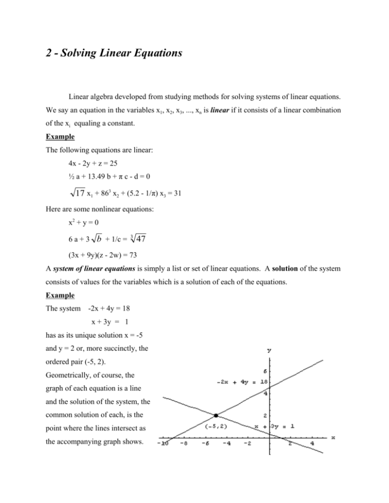
2 - Solving Linear Equations
Linear algebra developed from studying methods for solving systems of linear equations.
We say an equation in the variables x1, x2, x3, ..., xn is linear if it consists of a linear combination
of the xi equaling a constant.
Example
The following equations are linear:
4x - 2y + z = 25
½ a + 13.49 b + π c - d = 0
17 x1 + 863 x2 + (5.2 - 1/π) x3 = 31
Here are some nonlinear equations:
x2 + y = 0
6 a + 3 b + 1/c =
3
47
(3x + 9y)(z - 2w) = 73
A system of linear equations is simply a list or set of linear equations. A solution of the system
consists of values for the variables which is a solution of each of the equations.
Example
The system -2x + 4y = 18
x + 3y = 1
has as its unique solution x = -5
and y = 2 or, more succinctly, the
ordered pair (-5, 2).
Geometrically, of course, the
graph of each equation is a line
and the solution of the system, the
common solution of each, is the
point where the lines intersect as
the accompanying graph shows.
Problem
What other possibilities (geometrically) are there for the solution of a linear system with two
variables and two equations? What if there are three equations? Or just one?
Example
The following system with three variables
10x - 3y + 5z = 36
7x + 11y - 20z = -11
has the point (3, 8, 6) as one solution. Each equation has a plane as its graph as we see below.
Problem
What other solutions does this system have? What other possibilities (geometrically) are there for
the solution of a linear system with three variables and two equations? What if there are three
equations?
It is convenient to write the general system of linear equations using double subscripts for
the coefficients of the variables.
a11 x1 + a12 x2 + ... + a1n xn = b1
a21 x1 + a22 x2 + ... + a2n xn = b2
#
am1 x1 + am2 x2 + ... + amn xn = bm
The first subscript of each constant indicates the equation in which it is found, while the second tells
which variable it multiplies. All of the information of the system is contained in these constants so
we have the following definitions.
Definitions
1.
A matrix is a rectangular array of numbers. The size of a matrix with m rows and n columns
is m×n (read m by n.)
2.
The coefficient matrix of the system above is the matrix, A, whose i,j th entry (i.e., entry in
the ith row and jth column) is aij. As a shorthand we shall write A = (aij).
3.
The augmented matrix of the system consists of its coefficient matrix along with an
additional column, its (n+1)st, whose entries are the constants on the right-hand side of the
 b1 
 
b2
equations, so the last column is the vector b =   .
#
 
bm 
Example
The coefficient and augmented matrices of the system in the previous example with two variables
are
 −2
 −2 4

 and 
 1 3
1
4 18
 respectively.
3 1
Note that, for the general system that was given above, the first column of its coefficient
 a11 
 
a21 
matrix, c1 = 
, and, in general, its jth column, cj =
# 
 
 am1 
 a1 j 
 
 a2 j  , are vectors. For each i, the ith row
# 
 
 amj 
of the coefficient matrix, ri = (ai1 ai2 . . . ain), is also a vector and we can write the matrix in several
 r1 
 
r2
ways A = (aij) = (c1 c2 ... cn) =   . Using the vector operations introduced in the last chapter, we
#
 
 rm 
can form the linear combination of the columns of A and observe that x1, x2, ..., xn is a solution of
the system if and only if x1 c1 + x2 c2 + ... + xn cn = b, i.e. b is a linear combination of the columns
of A.
Example
Returning to the 2 × 2 example (2 equations with 2 unknowns) that we introduced earlier,
-2x + 4y = 18
x + 3y = 1 ,
we have as its corresponding equation with column vectors
 −2
 4
18
 , w =   , and b =   .
 1
 3
 1
x v + y w = b where v = 
Then the solution (-5, 2) can be pictured in the vector diagram that follows.
Thus we have two distinct pictures for systems, both of which have their value and to which we’ll
return. They are, as Strang refers to them in his text, the row picture (the intersecting lines shown
earlier) and the column picture (the linear combination of vectors in the graph above) of the system.
The latter picture was a result of viewing the system as a vector equation with the right hand side
of the system, b, written as a linear combination of the column vectors of the coefficient matrix.
With the dot product and the row expression of A, we can write the system
 x1 
 r1 ⋅ x 


 
 r2 ⋅ x  = b where x =  x2  .
 # 
 #


 
 rm ⋅ x
 xm 
Let’s exploit this view point in considering the possibilities for the system’s solutions.
We have seen from the row pictures with intersecting (and parallel) lines and planes that a
linear system can have no solution (in which case it is called inconsistent) or, if it is consistent, can
have a single, unique solution or infinitely many solutions. We now show that these are, in fact, the
only possibilities. Indeed, suppose that the general system has as distinct solutions the vectors x =
(x1, x2, ..., xn) and y = (y1, y2, ..., yn). Let z be the linear combination of x and y given by
z = t x + (1 - t) y
where t is an arbitrary real number. Consider for any i = 1, 2, .., m, the ith equation of the system.
Since x and y are solutions of the system (and, hence, each equation) ri · x = bi = ri · y . Then
ri · z = ri · (tx + (1 - t)y ) = t(ri · x) + (1 - t)(ri · y) = t bi + (1 - t) bi = bi. Thus z is a solution of the
ith equation for each i and so is a solution of the system. (Note: the second step in the string of
equalities uses the result of the problem below.)
Consequently any system with two distinct
solutions has infinitely many solutions. (Writing z = t x + (1 - t) y = y + t (x - y) it is not hard to
recognize that the terminal points of z drawn in standard position (with the origin as its initial point)
trace the line through the heads of the vectors x and y (in standard position) as the parameter t is
varied throughout the real numbers. This is the parametric form of the equation of this line.)
Problem
Show that the dot product is linear: for any vectors u, v, and w in Rn and any scalar c
1.
u · (v + w) = u · v + u · w
2.
v · (cw) = c(v · w)