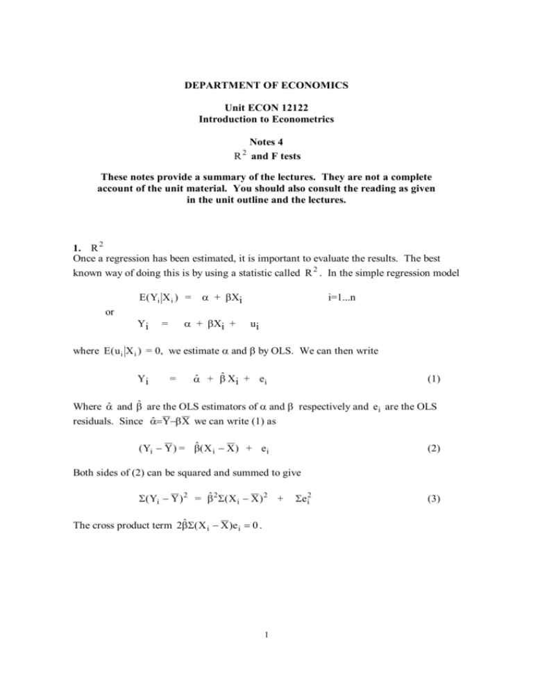
DEPARTMENT OF ECONOMICS
Unit ECON 12122
Introduction to Econometrics
Notes 4
R and F tests
2
These notes provide a summary of the lectures. They are not a complete
account of the unit material. You should also consult the reading as given
in the unit outline and the lectures.
1. R 2
Once a regression has been estimated, it is important to evaluate the results. The best
known way of doing this is by using a statistic called R 2 . In the simple regression model
E( Yi X i ) =
or
Yi
α + βXi
α + βXi +
=
i=1...n
ui
where E( u i X i ) = 0, we estimate α and β by OLS. We can then write
Yi
=
α̂ + β̂ Xi + e i
(1)
Where α̂ and β̂ are the OLS estimators of α and β respectively and e i are the OLS
residuals. Since αˆ=Y− βX we can write (1) as
( Yi − Y ) = βˆ( X i − X ) + e i
(2)
Both sides of (2) can be squared and summed to give
Σ( Yi − Y ) 2 = βˆ2 Σ( X i − X ) 2 +
The cross product term 2βˆΣ( X i − X )e i = 0 .
1
Σe i2
(3)
Equation (3) is an important relationship. Each term is referred to as a kind of sum of
squares.
Σ( Yi − Y ) 2
βˆ2 Σ( X i − X ) 2
Total sum of squares (TSS)
Σe i2
Residual sum of squares (RSS)
Explained sum of Squares (ESS)
Thus (3) says
TSS
=
ESS
+
R 2 is defined in the following way
RSS
ESS
TSS
R2 =
Because of (3) 0 ≤ R 2 ≤1
R 2 is often regarded as the “proportion of the variance of the dependent variable which
is explained by the regression line”. As such a higher value of R 2 is regarded as better
than a lower value. Unfortunately adding spurious explanatory variables to the
regression will always raise R 2 when the OLS technique is used to estimate the
coefficients. Thus a “high” value of R 2 is not always a good sign. In practice it is often
easy to find comparatively high values of R 2 in regressions using time series samples
and in this context R 2 is not very informative. Lower values of R 2 generally occur in
regressions using large cross-section samples and in this context R 2 is more useful.
Although see remarks on “the F test” below.
2. F tests
Whenever we wish to test a null hypothesis which contains restrictions on more than one
coefficient or consists of more than one linear restriction, a convenient test statistic has
the F distribution if the null hypothesis is true.
Suppose the model is
Yi = α 0 + α1X1i + α 2 X 2i + α 3X 3i + u i
examples of such null hypotheses would be
(i) α1 = 0, α 2 = 0 or
(ii) α1 + α 2 + α 3 = 1
2
i = 1,2,..,n
(4)
The F test procedure compares the value of RSS under the null (that is when the model is
restricted by the null) with the RSS when the model is unrestricted. Thus the restricted
model under the null of (i) above would be
Yi
=
α0 +
α 3X 3i + u i
i = 1,2,..,n
The formula for the F test is then
( RSS R − RSS U ) / d
RSS U ( n − k )
(5)
is distributed as F with d and (n-k) degrees of freedom.
Where RSS R is the RSS from the restricted equation
RSS U is the RSS from the unrestricted equation
d is the number of restrictions
n is the number of observations
k is the number of coefficients in the unrestricted equation.
Thus if the null was as in (i) above d = 2 and k = 4.
F tests can be used to test any linear restriction of the coefficients of a regression model.
It is important to remember that (5) only has the appropriate F distribution under the null
when certain assumptions about the regression model are true. These are
(i)
The model as described under H 0 is true.
(ii) E(uiuj) = σ2
i=j
(homoscedasticity)
= 0
i≠j
(no serial correlation)
(
)
(iii) either u i ~ N ο, σ2 or a sufficiently large sample for the central limit
theorem to apply.
3. Production Function Example
In Notes 2, a Cobb-Douglas production function was estimated on a sample of annual
data for UK manufacturing. The OLS results were these
yt
=
2.776 + 0.284 k t + 0.007 l t
(5.030)
(0.499)
(0.251)
+
et
t = 1,2,..,n
(6)
standard errors in brackets, n = 24, e t is the regression residual, R 2 = 0.1263, s = 0.0782,
RSS = 0.1283, F = 1.518
A number of diagnostic statistics have now been included.
3
R 2 indicates that by the standard of time series regressions, the regression line
“explains” a comparatively small proportion of the variation in log output. This is not
surprising given the fact the neither slope coefficient is estimated very precisely (both
estimated slopes have comparatively large standard errors).
s is an estimate of the standard error of the residuals. It is sometimes called the “standard
error of the regression”. It is calculated in the following way;
s=
2
∑ et
=
(n − k )
2
∑ et
21
In models where all the variables are measured in logs (as here), s has the interpretation
that it is a measure of the size of the average residual as a percentage of the dependent
variable. If this regression was used to predict the value of log output over the sample
period then the prediction would (on average) be wrong by 7.81 per cent.
RSS is the residual sum of squares. It will have a straightforward relationship with s
above. You should check that it does so.
F is “the F statistic” see section 4 below.
Now the reason why we were interested in estimating this Cobb-Douglas production
function was to test the hypothesis of constant returns to scale. The model is
y = A + α1 k + α 2 l + u
Where y = log(Y), A = log( α 0 ), k = log(K), l = log(L) and the random disturbance, u
with E(uk,l) = 0 and the hypothesis of constant returns to scale is α1 + α 2 = 1 . This is
the sort of hypothesis which the F test is designed for. To calculate the appropriate F
statistic we need RSS U and RSS R . We already have the RSS U from equation (6)
above (0.1283). We need RSS R . In practice this can often be computed by whatever
computer programme we are using. (See Exercise 7). In this example it turns out that
RSS R is 0.1339. Note that RSS R is larger than RSS U . If it was not, there would be
something wrong with the calculations. We can now compute the F statistic using
equation (5) above.
F=
(0.1339 − 0.1283) / 1
= 0.9166
0.1283 / 21
This F statistic has 1 and 21 degrees of freedom. The critical value of F(1,21) at 95 % is
4.32. Thus we cannot reject the null hypothesis that α1 + α 2 = 1 . As we have seen in
4
Notes 2, the 95 % confidence interval for α1 included one, so it is not perhaps a surprise
that we cannot reject the null of constant returns to scale.
4. Tests of Significance.
Often when a regression model is estimated, the investigator examines each of the
estimated coefficients to see if they are “significant”. This means testing the null
hypothesis that the coefficient is zero. The test statistic is
βˆ − 0
βˆ
=
which has a t distribution of (n-k) degrees of freedom.
s.e.(βˆ)
s.e.(βˆ)
This is often called “the t ratio” and is sometimes given in regression results in brackets
under the estimated coefficients instead of the standard error. It is important to realize
that it can be misleading to focus exclusively on the t ratio. A t ratio may be less than its
critical value (and thus the null is not rejected) because the standard error is large even
though the point estimate of β ( β̂ ) is also comparatively large.
On another occasion the point estimate may be comparatively small (0.002 say) but
because the standard error is even smaller, the estimated coefficient may be “significant”
(i.e. the null that the coefficient is zero is rejected). If, in the context of the model 0.002
is a very small effect, the fact that this particular coefficient is “significant” may not be
very interesting.
It is important to remember the that a confidence interval may give more information
about the range of possible values of the coefficient than a test of significance.
Just as there is “the t ratio” which tests the significance of one coefficient in a regression,
so there is “the F test” which tests the significance of all the slope coefficients in the
regression. Returning to the example given above, suppose the model is
Yi = α 0 + α1X1i + α 2 X 2i + α 3X 3i + u i
i = 1,2,..,n
(7)
We can test the joint null that
H 0 : α1 = 0, α 2 = 0, α 3 = 0 against
H 1 : any α i ≠ 0 for i = 1,2,3
The test statistic uses the formula (5) above. In this case the RSS U is the RSS from the
OLS estimate of the equation (6). The restricted equation takes the form
Yi = α 0 + u i
i = 1,2,..,n
5
and the RSS from this equation is the TSS from (6). This gives “the F statistic” a
particular form which is related to the R 2 from the unrestricted equation.
(TSS − RSS U ) /(k − 1)
R 2 /( k − 1)
“the F statistic” =
=
RSS U ( n − k )
(1 − R 2 ) /(n − k )
Often “the F statistic” is given as a diagnostic statistic with the regression results. For an
example of this see the estimates of the production function, equation (6) above. There
“the F statistic” is given as 1.518. This has a distribution of 2 and 21 degrees of freedom.
The critical value at 95 % is 3.47. Thus we do not reject the hypothesis that both α1 and
α 2 are zero. Again this is not very surprising since the 95% confidence intervals for
both these coefficients included zero (see Notes 2).
The link between R 2 and “the F statistic” provides a further interpretation to R 2 . If R 2
is comparatively high, it is more likely that the null that all the slope coefficients in the
regression are zero will be rejected. If it is comparatively low, then it is more likely that
this null will not to be rejected. Notice that “the F statistic” (like all F statistics) depends
on the number of observations (n) and the number of coefficients in the model (k). R 2
does not depend on n or k and thus can be artificially boosted as described in section 1
above. The reservations concerning the use of “the t ratio” given above also apply to “the
F statistic”.
5. Chow Tests
A special and useful application of the F test procedure is to test in time series models for
a “structural break”. A structural break is when the coefficients of the model change.
Thus suppose we have the following model
Yi = α 0 + α1X1i + α 2 X 2i + u i
i =1,2,..,T
(8)
It is believed that the coefficients may have changed at some point in the sample, say
after period s. If this were true we would have
Yi = β0 + β1X1i + β2 X 2i + u i
i =1,2,..,s
Yi = γ
0 + γ
1 X1i + γ
2 X 2i + u i
i =s+1,..,T
Note that the null hypothesis is
H 0 : no structural break after observation s.
H1 : structural break after observation s
6
and
(9)
(10)
Thus the restricted model is model (8) and the OLS estimates of that model provide
RSS R . The unrestricted model is equations (9) and (10). The RSS U is the sum of the
RSS for equation (9) and for equation (10). We then apply the formula for the F test as
given in (5). In this case it becomes
( RSS R − RSS U ) / k
RSS U (T − 2k )
which is distributed as F with k and (T-2k) degrees of freedom. Or in the example above
F with 2 and (T-4) degrees of freedom.
Note that this test requires that the point s is so placed in the sample that there are enough
observations both before and after s for the model to be estimated in each part. If this is
not true another form of the test is available (see the textbooks).
The test assumes that the variance of the disturbances is the same in both parts of the
sample. It is worthwhile checking that the estimates of the variance of the disturbances
from each part of the sample are not different by an order of magnitude. If the estimated
variances are different by that kind of margin, the Chow test will probably not be valid.
6. Examples of F tests
The following estimates were made with a sample of quarterly observations on UK data
1964.1-1991.3. The dependent variables is the log of consumers’expenditure on
consumption goods at 1985 prices. y is the log of disposable income at 1985 prices.
(I)
(ii)
(iii)
(iv)
Constant
-0.105
(0.176)
-0.149
(0.181)
0.738
(0.514)
-1.045
(0.337)
Yd t
1.249
(0.143)
1.004
(0.017)
0.946
(0.212)
1.502
(0.186)
Yd t − 1
0.185
(0.151)
-
0.178
(0.213)
-0.604
(0.182)
Yd t − 2
-0.434
(0.144)
-
-0.203
(0.210)
-0.603
(0.182)
R2
s
RSS
n
0.973
0.034
0.1237
111
0.971
0.035
0.1335
111
0.890
0.035
0.0564
50
0.951
0.030
0.051
61
Standard errors given in brackets.
7
The model being estimated here can be written
c t = a 0 + a1 y t + a 2 y t − 1 + a 3 y t − 2 + u t
t=1,2,… ,T
where c t is the log of consumers’expenditure at constant prices, y t is the log of
disposable income at constant prices. We will use the F test to test two different
hypotheses.
(i)
H 0 : a 2 = 0, a 3 = 0
H 1 : either a 2 ≠ 0 or a 3 ≠ 0
Using the estimates given above RSS U = 0.1237 and RSS R = 0.1335
Thus,
F=
(0.1335 − 0.1237) / 2
= 4.23
0.1237 / 107
This has an F distribution of 2 and 107 degrees of freedom. The 95% critical
value is 3.09 (approximately). Thus we reject the null hypothesis.
(ii)
Using the estimates given above we can also test for structural change after the
50th observation, that is after 1976.2.
H 0 : no structural break after observation 1976.2.
H1 : structural break after observation 1976.2.
For this test RSS U = 0.0564 + 0.051 = 0.1074 and RSS R = 0.1237
Thus,
F=
(0.1237 − 0.1074) / 4
= 3.91
0.1074 / 103
This has an F distribution of 4 and 103 degrees of freedom. The 95% critical
value is 2.46 (approximately). Thus we reject the null hypothesis that this form of
the consumption function did not have a structural break after 1976.2.
It is also important to check that the variance of the disturbances did not change at
the break point. The estimate of the variance for the first part of the sample is
0.0564/46 = 0.0012. In the second half of the sample it is 0.051/57 = 0.0009.
Although these estimates are not identical, they do not indicate that the variance
has substantially changed.
David Winter
March 2000
8