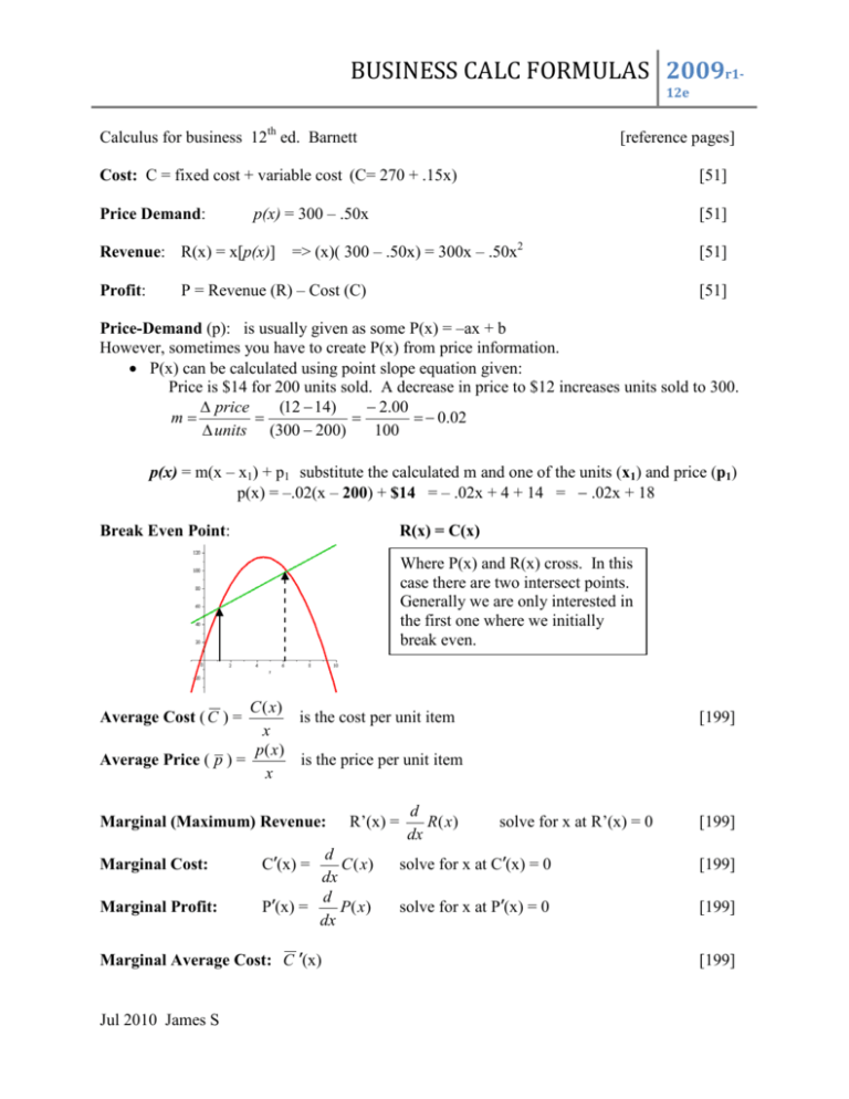
BUSINESS CALC FORMULAS 2009r112e
Calculus for business 12th ed. Barnett
[reference pages]
Cost: C = fixed cost + variable cost (C= 270 + .15x)
[51]
Price Demand:
[51]
p(x) = 300 – .50x
Revenue: R(x) = x[p(x)]
Profit:
=> (x)( 300 – .50x) = 300x – .50x2
P = Revenue (R) – Cost (C)
[51]
[51]
Price-Demand (p): is usually given as some P(x) = –ax + b
However, sometimes you have to create P(x) from price information.
• P(x) can be calculated using point slope equation given:
Price is $14 for 200 units sold. A decrease in price to $12 increases units sold to 300.
∆ price
(12 − 14)
− 2.00
=
=
= − 0.02
m=
∆ units (300 − 200)
100
p(x) = m(x – x1) + p1 substitute the calculated m and one of the units (x1) and price (p1)
p(x) = –.02(x – 200) + $14 = – .02x + 4 + 14 = − .02x + 18
Break Even Point:
R(x) = C(x)
Where P(x) and R(x) cross. In this
case there are two intersect points.
Generally we are only interested in
the first one where we initially
break even.
C ( x)
is the cost per unit item
x
p( x)
Average Price ( p ) =
is the price per unit item
x
Average Cost ( C ) =
Marginal (Maximum) Revenue:
Marginal Cost:
Marginal Profit:
d
C (x)
dx
d
P’(x) =
P(x)
dx
C’(x) =
Marginal Average Cost: C ’(x)
Jul 2010 James S
R’(x) =
d
R (x)
dx
[199]
solve for x at R’(x) = 0
[199]
solve for x at C’(x) = 0
[199]
solve for x at P’(x) = 0
[199]
[199]
BUSINESS CALC FORMULAS 2009r112e
− p f ' ( p)
p
p( x)
=
=
p'
xp'
f ( p)
Elasticity: E(p) =
[258]
Demand as a function of price: x = f (p)
E(p) = 1
E(p) > 1
E(p) < 1
unit elasticity (demand change equal to price change)
elastic (large demand change with price)
inelastic (demand not sensitive to price change)
x = f(p) = 10000 – 25p2
Find domain of p:
set f(p) ≥ 0
10000 – 25p2 ≥ 0
p2 ≤ 400
0 ≤ p ≤ 20
𝑓𝑓 ′ (𝑝𝑝) = −50𝑝𝑝
Find where E(p) is 1:
−𝑝𝑝𝑓𝑓 ′ (𝑝𝑝)
E(p) = �
p
E(p)
0
𝑓𝑓(𝑝𝑝)
50𝑝𝑝 2
−(𝑝𝑝)(−50(𝑝𝑝))
� = �10000 −25(𝑝𝑝)2 � = �10000 −25(𝑝𝑝)2 � = 1
=> 50p2 = 10000–25p2 => 75p2 = 10000 => p2 = 133.3
p = √133.3 = 11.55
(remember there is no negative value for p)
20
<1
=1
>1
Relative Rate of Change (RRC)
𝑓𝑓 ′ (𝑥𝑥)
𝑓𝑓(𝑥𝑥)
[256]
(find the derivative of f(x) and divide by f(x))
Also can be found with the dx( ln (f(p))
1
Demand RRC = dp [ ln (f(p)) ]
dx [ ln x ] = 𝑥𝑥 𝑑𝑑𝑑𝑑
Price RRC = f(x) = 10x+500
ln f(x) = ln [10x+500] = ln 10 + ln (x+50)
(log expansion)
1
1
dx [f(x)] = 𝑥𝑥+50 𝑑𝑑𝑑𝑑 = 𝑥𝑥+50
( ln10 is a constant so dx ln(10) = 0 )
Jul 2010 James S
[259]
BUSINESS CALC FORMULAS 2009r112e
Future Value of a continuous income stream:
𝐹𝐹𝐹𝐹 =
𝑇𝑇
𝑒𝑒 𝑟𝑟𝑟𝑟 ∫0 𝑓𝑓(𝑡𝑡)𝑒𝑒 (−𝑟𝑟𝑟𝑟 )
[424]
𝑑𝑑𝑑𝑑
Continuous income flow 𝑓𝑓(𝑡𝑡) = 500𝑒𝑒 0.04𝑡𝑡
Future value: 12%
Time: 5 yrs
5
𝐹𝐹𝐹𝐹 = 500𝑒𝑒 (.12)(5) � 𝑒𝑒 0.04(𝑡𝑡) 𝑒𝑒 −.12(𝑡𝑡)
0
FV = $3754
Surplus:
𝑥𝑥̅
PS (producer’s surplus) = ∫0 [ 𝑝𝑝̅ − 𝑆𝑆(𝑥𝑥)] 𝑑𝑑𝑑𝑑
CS (consumer’s surplus)
𝑥𝑥̅
= ∫0 [
Equilibrium is when: PS = CS
x is the current supply
5
𝑒𝑒 −.08𝑡𝑡
.6
𝑑𝑑𝑑𝑑 = 500𝑒𝑒 �
�
−.08 0
[426]
𝐷𝐷(𝑥𝑥) − 𝑝𝑝̅ ] 𝑑𝑑𝑑𝑑
p is the current price
𝑦𝑦�
𝑦𝑦�
𝑥𝑥̅
𝑥𝑥̅
Case A
Case B
𝑥𝑥̅
The surplus is the area between the curve [∫0 𝑓𝑓(𝑥𝑥) ] and the area of the box created by the
equilibrium point ( (𝑥𝑥̅ 𝑡𝑡𝑡𝑡𝑡𝑡𝑡𝑡𝑡𝑡 𝑓𝑓(𝑥𝑥̅ ) ). In Case A it is the (area of the box) – ( the area under the
curve); in Case B it is the (area under the curve) – ( area of the box).
Gini Index:
1
1
1
2 ∫0 �𝑥𝑥 − 𝑓𝑓(𝑥𝑥)� = 2 ∫0 𝑥𝑥 − 2 ∫0 𝑓𝑓(𝑥𝑥)𝑑𝑑𝑑𝑑
of f(x) separately and then subtract it from
Index is between 0 and 1.
Jul 2010 James S
1
2 ∫0 𝑥𝑥
You can solve the integral
which = 1. So essentially it is 1 −
[416]
1
2 ∫0 𝑓𝑓(𝑥𝑥).