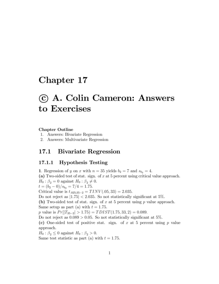
Chapter 17
c A. Colin Cameron: Answers
°
to Exercises
Chapter Outline
1. Answers: Bivariate Regression
2. Answers: Multivariate Regression
17.1
Bivariate Regression
17.1.1
Hypothesis Testing
1. Regression of y on x with n = 35 yields b2 = 7 and sb2 = 4.
(a) Two-sided test of stat. sign. of x at 5 percent using critical value approach.
H0 : β 2 = 0 against H0 : β 2 6= 0.
t = (b2 − 0)/sb2 = 7/4 = 1.75.
Critical value is t.025;35−2 = T IN V (.05, 33) = 2.035.
Do not reject as |1.75| < 2.035. So not statistically significant at 5%.
(b) Two-sided test of stat. sign. of x at 5 percent using p value approach.
Same setup as part (a) with t = 1.75.
p value is P r[|T35−2 | > 1.75) = T DIST (1.75, 33, 2) = 0.089.
Do not reject as 0.089 > 0.05. So not statistically significant at 5%.
(c) One-sided test of positive stat. sign. of x at 5 percent using p value
approach.
H0 : β 2 ≤ 0 against H0 : β 2 > 0.
Same test statistic as part (a) with t = 1.75.
1
c A. COLIN CAMERON: ANSWERS TO EXERCISES
2 CHAPTER 17. °
Critical value is t.05;35−2 = T INV (.10, 33) = 1.692.
Reject as 1.75 > 1.692. So statistically significant at 5%.
(d) One-sided test of stat. sign. of x at 5 percent using p value approach.
Same setup as part (c) with t = 1.75.
p value is P r[T35−2 > 1.75) = T DIST (1.75, 33, 1) = 0.045.
Reject as 0.045 < 0.05. So statistically significant at 5%.
(e) Two-sided test at 10 percent of whether or not slope coefficient equals 1.
H0 : β 2 = 1 against H0 : β 2 6= 1. t = (b2 − 1)/sb2 = (7 − 1)/4 = 1.50.
Critical value is t.05;35−2 = T INV (.10, 33) = 1.692.
Do not reject as |1.50| < 1.692. So not statistically different from 1 at 10%.
17.1.2
Coefficient estimate, standard error and t statistic
2.(a) b2 = 10 and t = 4. Calculate sb2 , the slope coefficient.
Since t = b2 /sb2 it must be that sb2 = b2 /t = 10/4 = 2.5.
(b) b2 = 10 and p = 0.0575. Calculate the t statistic. n = 35.
The p value is the combined area in the left-hand and right-hand tails. This
is 0.0575.
Now t.0575;35−2 = T IN V (.0575, 33) = 1.968.
The t statistic is 1.968.
17.1.3
R-Squared
3. n = 37 and R2 = 0.4.
(a) For regression of y on just one regressor x the R2 equals
√ the squared correlation coefficient. Thus the correlation coefficient r = ± 0.4 = ±0.632. Note
that we do not know the sign of the correlation coefficient without information
in addition to R2 .
(b) 40 percent of the variance of y is explained by regression on x.
(c) If s2y = 100 whatPis T SS, the total sum of squares of y?
n
1
1
2
In general s2y = n−1
i=1 (yi − ȳ) = n−1 T SS.
1
Here 100 = 36
T SS implies T SS = 36 × 100 = 3600.
(d) Given R2 = 0.40 and part (c), calculate ESS, the error sums of squares.
In general R2 = 1 − ESS/T SS.
Here 0.4 = 1−ESS/3600 implies ESS/3600 = 0.6 implies ESS = 0.6×3600 =
2160.
17.1. BIVARIATE REGRESSION
17.1.4
3
Inflation and Money Supply Growth
Annual data from 1960 to 1998. n = 39.
y =INFL. x =GM2. ȳ = 4.19, s2y = 6.19. x̄ = 7.12, s2x = 9.32.
y = 2.094 + 0.295x. R2 = 0.13.
1. GM 2t = 100 × (M 2t − M 2t−1 )/M 2t−1 .
2. Money supply growth is more volatile as it has larger variance, since 9.32 >
6.19.
3. Yes. Significant at 5 percent since p = 0.024 < 0.05.
Or more work is |t| = 2.361 > t.025;39−2 = T INV (0.05, 37) = 2.026.
4. dy/dx = dIN F L/dGM 2 = b2 = 0.295. A one percent increase in the
growth rate of M2 is associated with a 0.295 percent increase in the inflation
rate.
5. Question is asking whether or not the slope coefficient equals one.
Test H0 : β 2 = 1 against H0 : β 2 6= 1 at 5 percent.
t = (b2 − 1)/sb2 = (0.295 − 1)/0.1249 = −0.705/0.1249 = −5.645.
Critical value is t.05;39−2 = T INV (.05, 37) = 2.026. Reject H0 as 5.645 >
2.026.
Or p = Pr(|Tn−2 | > 5.645) = T DIST (5.645, 37, 2) = 1.90 × 10−6 < 0.05.
Reject H0 .
Either way yields reject H√
0 . Conclude that statistically different from one.
2
6. No. R = .13 and r = 0.13 = 0.36 are low. Not highly correlated.
7. The regression cannot discriminate between the two theories as it does not
establish causation.
17.1.5
Okun’s Law
Annual data from 1960 to 1998. n = 39.
y =GDP growth rate. x =CHANGE IN UNEM. ȳ = 4.19, s2y = 6.19. x̄ = 7.12,
s2x = 9.32.
y = 0.0318 − 1.951x.
1. GDP growtht = 100 × (GDPt − GDPt−1 )/GDPt−1 .
2. Yes. Significant at 5 percent since p = 4.43 × 10−11 < 0.05.
Or more work is |t| = 9.184 > t.025;39−2 = T DIST (0.05, 37) = 2.026.
Is the change in unemployment statistically significant at 5 percent?
3. Question is asking whether or not the slope coefficient equals −2.
Test H0 : β 2 = −2 against H0 : β 2 6= −2 at 5 percent.
t = (b2 − −2)/sb2 = (−1.951 − −2)/0.212 = −0.049/0.212 = −0.23.
c A. COLIN CAMERON: ANSWERS TO EXERCISES
4 CHAPTER 17. °
Critical value is t.05;39−2 = T INV (.05, 37) = 2.026.
Do not reject H0 as 0.23 < 2.026.
Or p = Pr(|Tn−2 | > 0.23) = T DIST (0.23, 37, 2) = 0.82 > 0.05.
Do not reject H0 .
Either way do not reject H0 . Conclude that not statistically different from −2.
4. Increase in unemployment rate from 5 percent to 7 percent in a year implies
change in unemployment rate equals 7 − 5 = 2.
Predicted yb = 0.0318 − 1.951 × 2 = −3.87.
Predicted reduction in the growth rate of real GDP is 3.87 percent.
17.2
Multivariate Regression
17.2.1
Hypothesis Testing
1. y = b1 + b2 x2 + b3 x3 with b2 = 20, t2 = 2.5, b3 = 40, t3 = 1.5. n = 40.
(a) Two-sided test of stat. sign. x2 and x3 at 5% using critical value approach.
H0 : β j = 0 against H0 : β j 6= 0.
Critical value is t.025;40−3 = T IN V (.05, 37) = 2.026.
For x2, t2 = 2.5 and |2.5| > 2.026. So x2 statistically significant at 5%.
For x3, t3 = 1.5 and |1.5| < 2.026. So x3 not statistically significant at 5%.
(b) Two-sided test of stat. sign. of x2and x3 at 5% using p value approach.
For x2, p value is P r[|T40−3 | > 2.5) = T DIST (2.5, 37, 2) = 0.017 < 0.05.
For x3, p value is P r[|T40−3 | > 1.5) = T DIST (1.5, 37, 2) = 0.142 > 0.05.
So x2 statistically significant at 5% and x3 not statistically significant at 5%..
(c) Test H0 : β 3 = 20 against H0 : β 3 6= 20 at 10 percent.
t = (b3 − 20)/sb3 .
The problem is what is sb3 ? Recall that t3 = b3 /sb3 , so here 1.5 = 40/sb3 . It
follows that sb3 = 40/1.5 = 26.67.
Thus t = (40 − 20)/26.67 = 0.75.
Critical value is t.05;39−2 = T INV (.05, 37) = 2.026.
Do not reject H0 as 0.75 < 2.026.
Or p = Pr(|Tn−2 | > 0.75) = T DIST (0.75, 37, 2) = 0.458 > 0.05.
Do not reject H0 .
Either way do not reject H0 . Conclude that not statistically different from −2.
17.2. MULTIVARIATE REGRESSION
17.2.2
5
F-test, R-squared and Adjusted R-squared
2. n = 35. Regress y on x2 yields R2 = 0.40 with k = 2. Regress y on x2 and
x3 yields R2 = 0.41 with k = 3.
(a) F test of whether or not x2 stat. sign. at 5% in regression of y on x2.
H0 : β 2 = 0 against Ha : β 2 6= 0.
F = [R2 /(k − 1)]/[(1 − R2 )/(n − k)] = [0.40/(2 − 1)]/[(1 − 0.40)/(35 − 2)] =
[0.40]/[0.60/33] = 22.
(b) F test of whether or not x2 and x3 are jointly stat. sign. at 5% in
regression of y on x2 and x3.
H0 : β 2 = 0, β 3 = 0 against Ha :At least one of β 2 6= 0, β 3 6= 0.
F = [R2 /(k − 1)]/[(1 − R2 )/(n − k)] = [0.41/(3 − 1)]/[(1 − 0.39)/(35 − 3)] =
[0.41/2]/[0.59/32] = 13.83.
(c) In genera R̄2 = R2 − [(k − 1)/(n − k)](1 − R2 ).
Just x2 : R̄2 = 0.40 −[(2 −1)/(35 −2)](1 −0.40) = 0.40 −[1/33]×0.60 = 0.382.
Both x2 and x3 : R̄2 = 0.41−[(3−1)/(35−3)](1−0.41) = 0.41−[2/32]×0.59 =
0.373.
Prefer the model with just x2 on the basis of R̄2 , as it has higher R̄2 .
17.2.3
Republican Voting
n = 50.
V OT EREP U B = 58.5814+0.27829×P OP CH−0.0014034×SCHOOL
(20.63)
(3.22)
(−2.24)
R2 = 0.258.
1. Yes. The two regressor variables are statistically significant at 5 percent.
Critical value is t.025;50−3 = T IN V (.05, 47) = 2.012.
2. Yes. The coefficients of POCCH and SCHOOL have the expected signs
and are statistically significant at 5 percent. (Here best to use a one-sided test
in which case the critical value is t.05;50−3 = T IN V (.10, 47) = 1.678).
3. Test H0 : β 2 = 0, β 3 = 0 against Ha :at least one β 2 , β 3 6= 0.
From formula sheet F = [R2 /(k − 1)]/[(1 − R2 )/(n − k)] = 8.17.
Yes. Reject H0 at 5 percent as F = 8.17 > F IN V (0.05, 2, 47) = 3.195.
or reject H0 at 5 percent as p = F DIST (8.171, 2, 47) = 0.0009 < 0.05.
4. Prediction for Canada is V OT EREP UB = 58.5814 + 0.27829 × 10 −
0.0014034 × 4000 = 55.75 > 50.00.
Yes. The model predicts that more than 50 percent would vote Republican.
c A. COLIN CAMERON: ANSWERS TO EXERCISES
6 CHAPTER 17. °
[A better answer would formally test whether the difference from 50 is statistically significant. There is not enough information here to do that.]
5. Positive: on average as income increases people are more likely to vote Republican. [This result may not necessarily hold once one controls for POPCH
and SCHOOL, but I expect it would.]
6. R2 always increases (or more precisely never decreases) when additional
regressors are added. So the increase is not a surprise. The question is whether
going from 0.250 to 0.270 is a big or small decrease.
7. Use R̄2 = R2 − [(k − 1)/(n − k)](1 − R2 ) which adjusts for model size.
Without income R̄2 = 0.258 − [2/47] × 0.742 = 0.226.
With income R̄2 = 0.270 − [3/47] × 0.730 = 0.223.
The model without income is preferred as R̄2 is larger.