We have seen that under Hardy-Weinberg conditions the genotypes AA, Aa , and aa will occur in the proportions p
2
, 2pq, and q
2
(where p + q = 1) after just one generation of random mating. This is a random association of alleles within genotypes. Consider a second autosomal locus with alleles B and b , with frequencies x + y = 1. It is common to observe that A is in random association with a , and B is in random association with b in the same population.
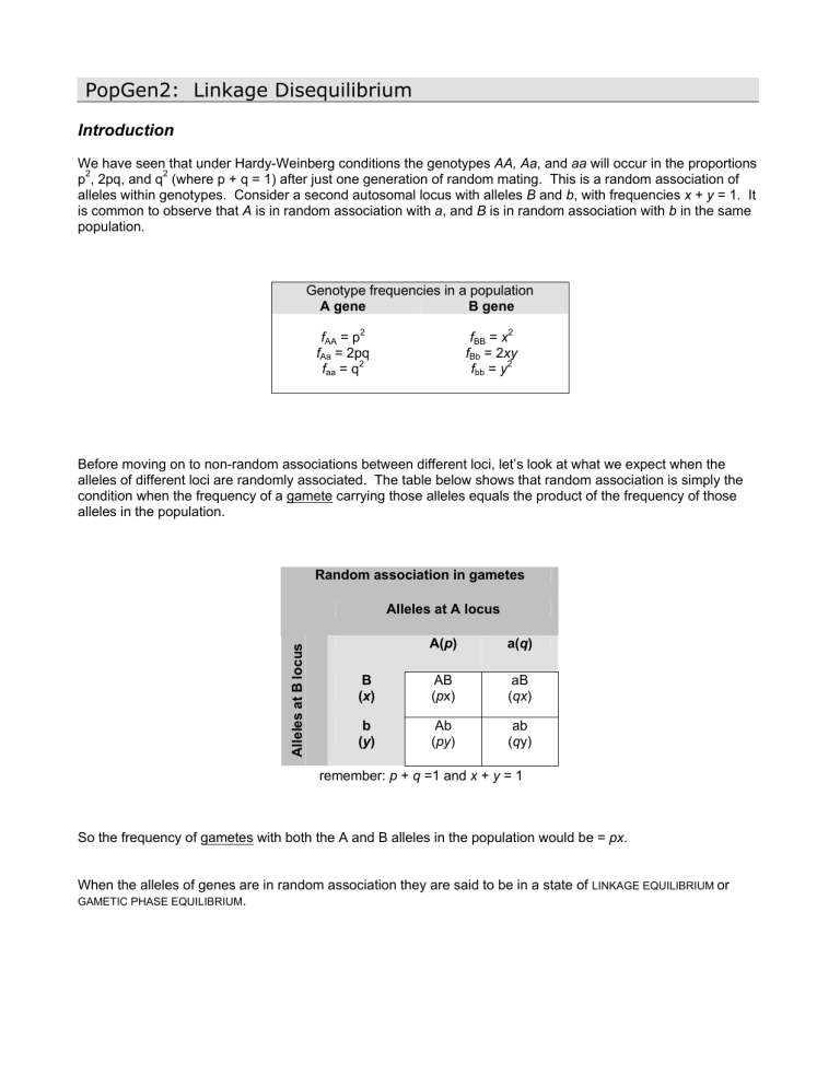
Genotype frequencies in a population
A gene B gene f
AA
= p
2 f
Aa f aa
= 2pq
= q
2 f
BB
= x
2 f
Bb f bb
= 2 xy
= y
2
Before moving on to non-random associations between different loci, let’s look at what we expect when the alleles of different loci are randomly associated. The table below shows that random association is simply the condition when the frequency of a gamete carrying those alleles equals the product of the frequency of those alleles in the population.
Random association in gametes
Alleles at A locus
A( p ) a( q )
B
( x ) b
( y )
(
(
AB p x)
Ab py )
(
( aB qx ab q
) y) remember: p + q =1 and x + y = 1
So the frequency of gametes with both the A and B alleles in the population would be = px .
When the alleles of genes are in random association they are said to be in a state of LINKAGE EQUILIBRIUM or
GAMETIC PHASE EQUILIBRIUM
.

What might be surprising is that it is common to observe that the alleles of gene A are not in random association with the alleles of gene B in the GAMETES , even though the alleles of each locus are in random association!
Let’s look at an example:
Population 1: 100% AABB
Population 2: 100% aabb
Suppose we mix these populations equally:
50% AABB and 50% aabb
After 1 generation of random mating and independent assortment we see the following:
AABB x AABB = AABB aabb x aabb = aabb
AABB x aabb = AaBb
We only see three of nine possible types: we don’t see any AaBB, aaBB, aaBb, AABb, AAbb, or Aabb!
They did not reach equilibrium after one generation of random mating.
With continued random mating the “missing” genotypes would appear, but not immediately at their equilibrium frequencies!
With two loci the attainment of equilibrium is gradual. In general, only about 50% of linkage disequilibrium is broken down each generation; hence, linkage disequilibrium can persist for a number of generations. This is in contrast to the attainment of Hardy-Weinberg proportions for a single locus, which can take just one generation of random mating!
It is easy to see that alleles of different genes might not be in random association and such cases are said to be in a state of GAMETEIC PHASE DISEQUILIBRIUM . The term LINKAGE DISEQUILIBRIUM or LD is used interchangeably with gametic phase disequilibrium.
Note that other factors can make the attainment of equilibrium frequencies take even longer. If two loci are physically linked on a chromosome then the appearance of the “missing” genotypes also depends on the rate of recombination between the loci. Physical linkage increases disequilibrium. Disequilibrium also can arise due to mixing populations with different allele frequencies, or even by chance in small populations.
In order to look at this more closely we need to use a modification of the standard genotypic symbolism. Take
. the genotypic symbolism for an AaBb individual as an example, the standard symbolism does not distinguish between two important cases:
Case 1: AB gamete + ab gamete = AaBb
Case 2: Ab gamete + aB gamete = AaBb
New symbolism:
AB/ab indicates the union of AB gamete + ab gamete

So, with our new system an individual of genotype AB/ab can produce four types of gametes:
(1) AB
(2) ab
Non recombinant gametes (same as in previous generation)
(3) Ab
Recombinant gametes (different from previous generation)
(4) aB
Frequencies of gametes ( f ) when genes are on different chromosomes: f
AB
= f ab
= f
Ab
= f aB f ( non-recombinant) = f (recombinant )
Frequencies of gametes ( f ) when genes are “linked” on same chromosome: f
AB
= f ab
≠ f
Ab
= f aB f ( non-recombinant)
≥ f (recombinant )
T he RECOMBINATION FRACTION ( r ) is the proportion of recombinant gametes produced by an individual. When genes are on different chromosomes, or when they are on the same chromosome and recombination is so frequent that recombination leads to independence of the two loci, then r = 0.5; i.e., f
Ab
+ f aB
= 0.5. An example of linkage with some recombination is provided below.
Individual AB/ab produces the following:
(1) AB: f
AB
= 0.38
(2) ab: f ab
= 0.38
(3) Ab: f
Ab
= 0.12
(4) aB: f aB
= 0.12 r = 0.12 + 0.12 = 0.24
Genes for which the recombination fraction (r) is less than 0.5 must necessarily be located on the same chromosome, and are said to be LINKED .
The recombination fraction is important in population genetics because the approach to equilibrium in the population depends on the values of r. At a value of r = 0.5 the alleles of different loci will be in equilibrium. As the recombination fraction decreases, the rate to equilibrium decreases; i.e., it takes even more generations of random mating than when r = 0.5. When r = 0, there is complete linkage (no recombinants ever appear) and so this population will be permanently in a state of disequilibrium with respect to the involved alleles.

Let’s consider the frequencies of the gamete types in a population: f
AB
+ f ab
+ f
Ab
+ f aB
= 1
We can define linkage equilibrium in the population under random association of the individual alleles.
Remember we defined f
A
= p and f a
= q and f
B
= x and f b
= y , where p + q = 1 and x + y = 1. Then based on the table above the equilibrium frequencies of the gametes are: f
AB
= p x f ab
= q y f
Ab
= py f aB
= qx
Suppose we know the actual frequency of AB gametes and we call it f
AB
. We can then compute the frequency of the AB gametes in the next generation; let’s call it f
AB
’. f
AB
' =
6
4
−
4 4
2 r
probabilit y of
7 no recombinat ion
4 4 f
4 frequency of
8
AB gametes in last generation
+
6
{
prob of
4 4 8 prob of putting recomb together A and B at random from recombinan ts
Subtract px from both sides gives: f
AB
' − px
=
− r
f
AB
− px
We can think in terms of the difference between the observed frequency of the AB gamete in the population and the expected equilibrium frequency ( f
AB
’
– px ) . Let’s call this difference D .
D
=
− r
f
AB
− px
The quantity D is called the LINKAGE DISEQUILIBRIUM PARAMETER . With random mating the value of D changes each generation according to the above formula. When D = 0 there is no more linkage disequilibrium, and the gamete frequencies observed in the present generation equal those predicted by the allele frequencies of the previous generation (e.g., f
AB
= px ).
The value of D holds for all four of the possible types of gametes: f
AB
= p x + D f ab
= q y + D f
Ab
= py - D f aB
= qx - D
So, the difference from equilibrium is positive (+ D ) for the non-recombinant types and negative for the recombinant types (D ).

It can be shown that D will satisfy the following equation:
D
= × f aa
− × f non recombinan t recombinan t
For any set of allele frequencies in a population ( p, q, and x, y ), we can compute the theoretical minimum ( D min
) and maximum ( D max
) values of D .
D min
= − px
− qy
D max
= + qx
+ py
The largest possible value of D is 0.25 [when all gametes are non-recombinant], and is only possible if p = q =
0.5. All other real values of D will be lower. Note it is possible to make D larger than 0.25, but this requires negative allele frequencies and that is clearly impossible.
More difficult is the comparison of D among populations that have different allele frequencies. To do this we can standardize the amount of disequilibrium as the fraction of the theoretical maximum for a population:
D
D max
Let’s look at a sample of 1000 people from Britain who were typed for the alleles at two different blood group loci: (i) the MN blood group and (ii) the Ss blood group. Let’s use p and q to denote the frequencies of the alleles at the MN locus and x and y for the frequencies of alleles at the Ss locus. The frequencies are as follows:
MN blood group f
M
= p = 0.5425 f
N
= q = 0.4575
Ss blood group f
S
= x = 0.3080 f s
= y = 0.6920
Gamete frequencies
MS = 474/2000 = 0.2370
Ms = 611/2000 = 0.3055
NS = 142/2000 = 0.0710
Ns = 773/2000 = 0.3865
We can ask “what is the amount of disequilibrium among these loci as a percentage of the theoretical maximum?”

The observed disequilibrium is D = (0.2370)(0.3865) – (0.3055)(0.0710) = 0.07.
The theoretical maximum come from D max
= qx = 0.14 or = py = 0.37, so D max
= 0.14
Hence, the observed disequilibrium is (0.07/0.14)*100 = 50% of the theoretical maximum.
Given the observed genotype frequencies, show that the MN and Ss loci are in Hardy-Weinberg equilibrium.
Genotype counts in the population
MN locus Ss locus
MM = 298
MN = 489
NN = 213
SS = 483
Ss = 418 ss = 99
Now use the chi-square test to determine if the observed gamete frequencies are in equilibrium. Hint: remember that because humans are diploid there are twice as many chromosomes as there are individuals, so the test is conducted by using the frequencies of the chromosomes!
As long as r > 0, D changes each generation until the gamete frequencies are at equilibrium. The recombination rate, and hence the fraction of recombinant genotypes produced in a generation, determines the rate at which equilibrium is approached. The closer r is to zero the slower the rate (see figure below).
Rate of decay of LD under various recombination rates
1
0.9
0.8
0.7
r= 0.001
0.6
0.5
r= 0.01
0.4
0.3
0.2
0.1
r= 0.5 r= 0.1
0
1 9 17 25 33 41 49 57 65 73 81 89 97 generations
Remember: r = 0.5 represents genes on different chromosomes, or genes sufficiently that are far apart on the same chromosome for independent assortment.

•
Migration : We saw this effect in our above example where we mixed two populations and saw an immediate disequilibrium effect. Any level of mixing of two populations with different frequencies, via migration of individuals from one population to another, will yield a disequilibrium effect. Because the breakdown of disequilibrium is slow the effect of even one round of mixing will persist for many generations. Population geneticists take advantage of this effect to study the process of migration between populations!
•
Natural Selection : Natural selection for combinations of alleles at different loci will maintain disequilibrium among loci, even in the face of frequent recombination.
•
Genetic Drift : In the above, equilibrium values were obtained by assuming infinitely large populations.
As we will see in a later topic, finite populations accumulate random fluctuation in allele frequencies from generation to generation. This process randomly associates alleles with each other. Hence there is a dynamic relationship between drift and recombination which will differ among populations of different sizes. Smaller sized populations will tend to have higher LD, but not always.
Identification of disease genes generally fall into one of two broad categories of methods. The traditional method uses family pedigrees. This method, called a F
AMILY STUDY
, looks for polymorphic markers that cosegregate on the family pedigree with the disease. Such co-segregation occurs when the marker is so close to the disease gene that the probability of recombination between the marker and the disease gene is very low.
This method relies on very high penetrance of the disease. In many cases the basis of the disease is more complex, being influenced by genetic interactions at several loci. Such diseases typically are more subject to non-genetic influences on the phenotype. The “signal” of such a disease in a pedigree will be quite low, requiring very large pedigrees in order to identify the candidate regions of the genome. Other problems with family studies include low map resolution and ascertainment bias towards loci that exhibit more typical Mendelian transmission patterns.
An alternative to the family study is a population based approach called LINKAGE DISEQUILIBRIUM MAPPING (or LD
MAPPING
), and sometimes called an
ALLELIC ASSOCIATION STUDY
, and it is applied to a population rather than a family pedigree. LD mapping is based on the fact that the mutation in the gene that is responsible for a disease arises on a particular chromosome, and over time recombination results in a strong LD signal only with those genetic variants that are very close, physically, to the disease causing gene. To conduct an LD mapping study, a sample of unrelated individuals that are both affected and unaffected are taken from a specific population. A set of genetic markers that are known to be highly polymorphic, such as SNPs or micro-satellites, are chosen that span a candidate region. The power of this approach comes from knowing where these polymorphic markers are located in a genome. You look for markers that exhibit strong disequilibrium of alleles with the disease trait. Association studies have their limitations as well. If the disease is influenced by rare alleles at many loci this approach will have low power. The recombination rate and the age of the mutation in the population affect the power of the approach.
We have only barely introduced the notion of LD in this session. However, it is an extremely important tool for identifying candidate disease genes, and highly sophisticated statistical methods based on maximum likelihood and Bayesian techniques have been developed to aid LD mapping.

The figure below illustrates the occurrence of a disease mutation in a population ( ) that is polymorphic. A subset of that population go off to start a new population and consequently the new population has a higher frequency of the founders genotypes and none of the genotypes that were not among the founders (this is called the founder effect; we will get back to it later in the course). The disease allele has a higher frequency in the new population. If it is recessive it can “hide” from natural selection in the heterozygotes as the CF allele does in
North America. Over time, recombination breaks up disequilibrium with all but the most tightly linked variants.
This is the point at which an association study might work well.
Disease mutation occurs in polymorphic population
Founder event increases freq of some genotypes; others are lost
Over time, recombination breaks association with more distant variants
•
With two loci, the attainment of equilibrium between alleles at different loci is gradual, being > 1 generation of random mating.
•
Physical linkage on the same chromosome slows the rate to equilibrium even more.
•
The recombination fraction determines the rate to equilibrium, the lower the fraction, the longer to equilibrium.
•
When in different chromosomes. When r < 0.5 the genes are said to be linked. When r =0 the loci are in permanent disequilibrium.
•
Disequilibrium can arise from sources other than linkage: o Admixture of populations o Natural selection acting on one or more of the loci o Inbreeding o Genes located in a chromosomal inversion ( SUPERGENE )
•
The LINKAGE DISEQUILIBRIUM is used to describe any source of disequilibrium, regardless of whether the two genes are physically linked or not.