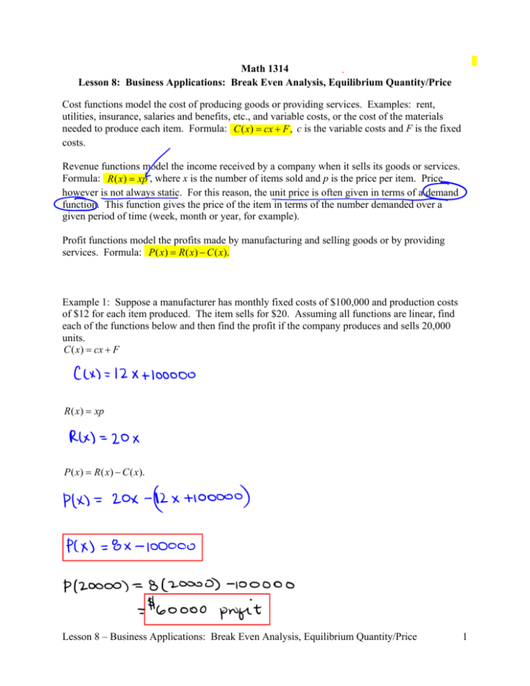
Math 1314
Lesson 8: Business Applications: Break Even Analysis, Equilibrium Quantity/Price
Cost functions model the cost of producing goods or providing services. Examples: rent,
utilities, insurance, salaries and benefits, etc., and variable costs, or the cost of the materials
needed to produce each item. Formula: C ( x)  cx  F , c is the variable costs and F is the fixed
costs.
Revenue functions model the income received by a company when it sells its goods or services.
Formula: R ( x )  xp , where x is the number of items sold and p is the price per item. Price
however is not always static. For this reason, the unit price is often given in terms of a demand
function. This function gives the price of the item in terms of the number demanded over a
given period of time (week, month or year, for example).
Profit functions model the profits made by manufacturing and selling goods or by providing
services. Formula: P ( x )  R ( x )  C ( x ).
Example 1: Suppose a manufacturer has monthly fixed costs of $100,000 and production costs
of $12 for each item produced. The item sells for $20. Assuming all functions are linear, find
each of the functions below and then find the profit if the company produces and sells 20,000
units.
C ( x)  cx  F
R ( x )  xp
P ( x )  R ( x )  C ( x ).
Lesson 8 – Business Applications: Break Even Analysis, Equilibrium Quantity/Price
1
Break-Even Analysis
The break-even point in business is the point at which a company is making neither a profit nor
incurring a loss. At the break-even point, the company has met all of its expenses associated
with manufacturing the good or providing the service. The x coordinate of the break-even point
gives the number of units that must be sold to break even. The y coordinate gives the revenues at
that production and sales level.
Example 2: Find the break-even point for the problem in Example 1.
Command:
Answer:
Lesson 8 – Business Applications: Break Even Analysis, Equilibrium Quantity/Price
2
You may be given raw data concerning costs and revenues. In that case, you’ll need to start by
finding functions to represent cost and revenue.
Example 3: Suppose you are given the cost data and demand data shown in the tables below.
quantity produced 50
100
200
500
1000
1200
1500
2000
total cost
100400 140100 182000 217400 229300 232600 239300 245500
quantity demanded 50 100 200 500 1000 1200 1500 2000
price in dollars
295 285 280 270 250 248 249 248
a. Find a linear regression equation that models costs, and a linear regression equation that
models demand. Begin by entering the data in GGB. Then create lists.
Linear Cost Model:
Command:
Answer:
Linear Demand Model:
Command:
Answer:
b. State the revenue function.
Command:
Answer:
c. Find the break-even point.
Command:
Answer:
Lesson 8 – Business Applications: Break Even Analysis, Equilibrium Quantity/Price
3
Market Equilibrium
Market equilibrium occurs when the quantity produced equals the quantity demanded. The
quantity produced at market equilibrium is called the equilibrium quantity and the
corresponding price is called the equilibrium price. Mathematically speaking, market
equilibrium occurs at the point where the graph of the supply function and the graph of the
demand function intersect. We can solve problems of this type either algebraically or by using
GGB.
Example 4: Suppose that a company has determined that the demand equation for its product is
5 x  3 p  30  0 where p is the price of the product in dollars when x of the product are
demanded (x is given in thousands). The supply equation is given by 52 x  30 p  45  0 , where
x is the number of units that the company will make available in the marketplace at p dollars per
unit. Find the equilibrium quantity and price.
Enter the functions into GGB as shown. If GGB does not like the variable “p” then replace it
with the variable “y” and proceed.
Command:
Answer:
Quantity:
Price:
Example 5: The quantity demanded of a certain electronic device is 8000 units when the price is
$260. At a unit price of $200, demand increases to 10,000 units. The manufacturer will not
market any of the device at a price of $100 or less. However for each $50 increase in price
above $100, the manufacturer will market an additional 1000 units. Assume that both the supply
equation and the demand equation are linear. Find the supply equation, the demand equation and
the equilibrium quantity and price.
Give two points for demand:
Give two points for supply:
Create two lists:
Commands:
Quantity:
Price:
Lesson 8 – Business Applications: Break Even Analysis, Equilibrium Quantity/Price
4