Topometric Localization on a Road Network
Topometric Localization on a Road Network
Danfei Xu
1
, Hern´an Badino
1
, and Daniel Huber
1
Abstract — Current GPS-based devices have difficulty localizing in cases where the GPS signal is unavailable or insufficiently accurate. This paper presents an algorithm for localizing a vehicle on an arbitrary road network using vision, road curvature estimates, or a combination of both. The method uses an extension of topometric localization, which is a hybrid between topological and metric localization. The extension enables localization on a network of roads rather than just a single, non-branching route. The algorithm, which does not rely on GPS, is able to localize reliably in situations where GPSbased devices fail, including “urban canyons” in downtown areas and along ambiguous routes with parallel roads. We demonstrate the algorithm experimentally on several road networks in urban, suburban, and highway scenarios. We also evaluate the road curvature descriptor and show that it is effective when imagery is sparsely available.
I. I NTRODUCTION
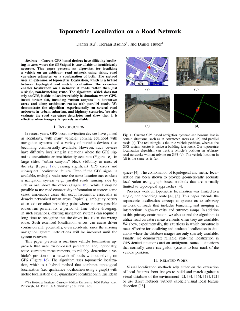
In recent years, GPS-based navigation devices have gained in popularity, with many vehicles coming equipped with navigation systems and a variety of portable devices also becoming commercially available. However, such devices have difficulty localizing in situations where the GPS signal is unavailable or insufficiently accurate (Figure
large cities, “urban canyons” block visibility to most of the sky (Figure
1 a), causing significant GPS errors and
subsequent localization failure. Even if the GPS signal is available, multiple roads near the same location can confuse a navigation system (e.g., parallel roads running side by side or one above the other) (Figure
possible to use road connectivity information to correct some cases, ambiguous cases still occur frequently, especially in densely networked urban areas. Typically, ambiguity occurs at an exit or other branching point where the two possible routes run parallel for a period of time before diverging.
In such situations, existing navigation systems can require a long time to recognize that the driver has taken the wrong route. Such extended localization errors can cause driver confusion and, potentially, even accidents, since the ensuing navigation system instructions will be incorrect until the system recovers.
This paper presents a real-time vehicle localization approach that uses vision-based perception and, optionally, route curvature measurements, to reliably determine a vehicle’s position on a network of roads without relying on
GPS (Figure
1 d). The algorithm uses topometric localiza-
tion, which is a hybrid method that combines topological localization (i.e., qualitative localization using a graph) with metric localization (i.e., quantitative localization in Euclidean
1
The Robotics Institute, Carnegie Mellon University, 5000 Forbes Ave.,
Pittsburgh, PA 15213 USA dhuber@cs.cmu.edu
(a)
(c)
(b)
(d)
Fig. 1: Current GPS-based navigation systems can become lost in certain situations, such as in downtown areas (a), (b) and parallel roads (c). The red triangle is the true vehicle position, whereas the
GPS system locates it inside a building (car icon). Our topometric localization algorithm can track a vehicle’s position on arbitrary road networks without relying on GPS (d). The vehicle location in
(d) is the same as in (a).
space) [4]. The combination of topological and metric localization has been shown to provide geometrically accurate localization using graph-based methods that are normally limited to topological approaches [4].
Previous work on topometric localization was limited to a single, non-branching route [4], [5]. This paper extends the topometric localization concept to operate on an arbitrary network of roads that includes branching and merging at intersections, highway exits, and entrance ramps. In addition to this primary contribution, we also extend the algorithm to utilize road curvature measurements when they are available.
We show, experimentally, the situations in which curvature is most effective for localizing and evaluate localization in situations where the database images are only sparsely available.
Finally, we demonstrate reliable, real-time localization in
GPS-denied situations and on ambiguous routes – situations that normally cause navigation systems to lose track of the vehicle position.
II. R ELATED W ORK
Visual localization methods rely either on the extraction of local features from images to build and match against a visual database of the environment [2], [3], [16], [17], [21] or use direct methods without explicit visual local feature detection [18].
The two main categories of visual localization approaches are metric and topological. Topological approaches [2], [3],
[21] use graphs in which nodes identify distinctive places of the environment and edges link them according to some distance or appearance criteria. Localization is achieved by finding the node where the robot is currently located.
Metric localization provides, instead, quantitative estimates of observer position in a map. Simultaneous localization and mapping (SLAM) [17], [18], and visual odometry [9], and some appearance-based localization approaches relying on accurate 3D maps [ ?
], [15] fall into this category.
The fusion of topological and metric localization has been approached before – mainly in the SLAM domain and using
3D sensors [7], [8], [14], [16], [20]. In these approaches, the fusion aims at segmenting metric maps represented by topological nodes in order to organize and identify submap relations and loop closures.
Recently, researchers have proposed fusing metric localization approaches with road trajectory information taken
from prior maps, such as OpenStreet 1 . Localization is
achieved by matching observed trajectories, constructed from visual odometry [9], [12] or IMU-based odometry [22], with a prior map using various techniques, such as Chamfer matching [12], curve similarity matching [22], or street segment matching [9]. Such approaches, however, are subject to drift in situations where the road geometry offers no constraints (e.g., long, straight road segments), particularly when visual odometry is used. Our probabilistic framework can incorporate road geometry features naturally, as we demonstrate with the curvature descriptor, but the visual localization provides complimentary constraints to prevent drift in most cases.
Our approach differs from visual SLAM methods that incrementally construct a map [11]. Those methods are typically more focused on accurate loop closure and topological correctness than accurate localization. For example, [11] reports any match within 40 meters of the true match as correct. In contrast, our approach reliably achieves average localization accuracy on the order of 1 m. On the downside, our approach requires a prior map to localize with respect to.
However, this is not such an onerous requirement, since such maps already exist (e.g., Google Street View). Our previous work has shown that the maps do not have to be updated very frequently, as localization is robust to changing conditions, such as seasonal variations and different weather and light conditions [5], [6].
III. L OCALIZATION O N A R OAD N ETWORK
The prior map needed for topometric localization is created by traversing the routes with a vehicle equipped with a similar (though not necessarily identical) set of sensors to those used at runtime. The next several sub-sections describe how the road network map is represented (Section
how it is automatically created (Section
metric localization for a non-branching route (Section
1 http://wiki.openstreetmap.org/wiki/planet.osm
Fig. 2: The road network is represented as a directed graph.
Edges correspond to road segments (yellow lines), and nodes connect edges at splitting and merging points (red dots). Intersection boundaries are denoted as white circles.
and the extension of topometric localization to road networks
(Section
A. Road Network Map Representation
A road network is represented by a directed graph G ( V, E )
(Figure
E in G correspond to segments of a road with no junctions. The direction of the edge indicates the direction of legal traffic flow. Vertices V in G correspond to points where road segments merge or split
(called “split points” and “merge points” hereafter). An intersection is represented by several edges in G , with each legal path through the intersection represented separately.
Lanes traveling in opposite directions on the same road are represented by separate edges as well. Each edge in G is subdivided into a linear sequence of fine-grained nodes, each of which is associated with a geographical location
(e.g., GPS coordinates) and a set of features derived from observations obtained at that location. The fine-grained nodes are spaced at constant intervals along the length of each edge.
B. Location Appearance and Road Curvature Descriptors
In this work, we use two types of descriptors. The location appearance descriptor is derived from camera imagery, and the road curvature descriptor is derived from the vehicle motion estimate.
Location appearance.
For encoding location appearance, the whole-image SURF (WI-SURF) descriptor has previously been shown to be robust to changes in lighting and environmental conditions [5]. The WI-SURF descriptor is an adaptation of the upright SURF (U-SURF) descriptor to cover an entire image [1]. It is a 64-vector encoding of the distribution of wavelet filter responses across the image. Each fine-grained node in the graph is associated with the WI-
SURF descriptor of the geographically closest observation.
Other, potentially more discriminitive, appearance descriptors, such as the bag of words used in FAB-MAP 2.0 [11], could be interchanged for the WI-SURF descriptor. However,
WI-SURF is much more computationally efficient, requiring only 0.45 ms to compute (enabling the full algorithm to easily run in real-time), as compared to extraction and computation of hundreds of SURF descriptors per image,
as required by FAB-MAP’s SURF/bag of words approach, which takes about 0.5 seconds to process and inhibits realtime operation [10].
Location curvature.
In this paper, we introduce a road curvature descriptor, which we hypothesize can aid in localization at splitting points, such as intersections and highway exits. The curvature descriptor models the curvature of the recent history of the vehicle’s route. Specifically, we define the descriptor as the signed difference in vehicle orientation
(yaw) at the current position and the orientation a fixed distance backward along the route: c i
= θ i
− θ i − L
, (1) where θ is the vehicle yaw (in radians), i indexes the current node in the map, and L is the lookback distance in nodes. The yaw is measured with respect to an arbitrary fixed orientation and is limited to the range − π/ 2 to π/ 2 .
The curvature descriptor is both computationally efficient and easily available. In our implementation, we use the vehicle’s IMU to compute the descriptor. However, if an IMU is not available, any means of estimating relative orientation can be used, such as a compass, a gyro, or integrating the steering wheel position. A descriptor is computed and stored for each fine-grained map node. The single scalar value adds negligible storage requirements to the map and is efficient to compute.
In our experiments (Section
termine a suitable lookback distance L and evaluate the benefits of using the curvature descriptor for localization.
As will be shown, the descriptor can significantly accelerate convergence to the correct route after passing a split point.
C. Automatic Road Network Map Creation
The road network map is created by driving a mapping vehicle along the routes that comprise the network, ensuring that each significant road segment is traversed at least once. As the vehicle drives the route, a route database is created, containing a sequence of fine-grained nodes spaced at uniform intervals (1 m in our implementation) along with observations from on board cameras and motion trajectory measurements. Location appearance and road curvature descriptors are computed using these observations and stored with each fine-grained node.
The initial map is a linear route with no concept of intersections or connectivity at split points or merge points.
The route may have redundant sections because the vehicle sometimes needs to traverse the same path multiple times to fully explore the entire route network. We process the initial map to remove these redundant sections and transform the route into a graph-based road network (Figure
intersections in the network are identified. Intersections can be detected using online digital maps (e.g., Google Maps) or by heuristics on the geometry of the node locations. For each intersection, a circle encompassing that intersection is defined. Each point where the vehicle route crosses this circle is detected, and a vertex is added to the road network graph
G . Directed edges are then added for each route segment connecting vertices in sequence along the traversed route.
Next, redundant edges are detected and eliminated. An edge is considered redundant if its source and sink vertices are both within a threshold distance of those from another edge.
It is not strictly necessary to traverse all segments within intersections, as it can be challenging to cover all possible routes through every intersection. Instead, missing segments through intersections are inferred. Each node representing an entrance to an intersection is connected to all other nodes representing departures from the intersection, with the exception of the route traversing the opposite direction on the same road (i.e., no u-turns allowed in intersections). Then a new segment is created for each inferred route through the intersection by fitting a b-spline connecting the two adjacent segments. Curvature descriptors are calculated for these inferred segments, but location appearance descriptors are not.
D. Topometric Localization on a Road Segment
Once a road network map is created, we use topometric localization to determine the location of the vehicle as it drives anywhere on the network at a later time. We first briefly review the basic topometric localization algorithm, which is limited to non-branching routes, and then demonstrate how it is extended to handle a road network. See [5] for details of the basic algorithm.
The vehicle position is represented as a probability distribution over fine-grained nodes and tracked over time using a discrete Bayes filter [19]. We chose the discrete Bayes filter over alternate approaches, such as a Kalman filter or a particle filter, because we wanted the algorithm to be capable of localizing globally, which is not achieved by a Kalman filter and is not guaranteed by a particle filter. At a given time t , the estimated position of the vehicle is a discrete random variable X t with possible values corresponding to finegrained nodes in the route (i.e., x k
, k = 1 , 2 , 3 ...N
, where
N is the number of nodes in the route). The probability of the vehicle being at node x k p k,t
= p ( X t
= x k
) at time t is denoted as and the probability distribution (pdf) over all nodes is p ( x k
) = { p k,t
} .
The position estimate pdf p ( x k
) is initialized to the uniform distribution or to a prior estimate of vehicle position, if available. The Bayes filter repeatedly updates the pdf by applying two steps: prediction , which incorporates the vehicle’s motion estimate; and update , which incorporates knowledge from new measurements. Formally,
Input : { p k,t − 1
Output : { p k,t
# Predict p k,t
= P
N i =1
# Update p k,t
}
} , s t
, z t p ( x k,t
| s t
= η p ( z t
| x k,t
, x i,t − 1 p k,t
= x i
) p i,t − 1 where s t and z t are the vehicle velocity and observations at time t respectively and η is a normalizing constant. To
0.07
0.06
0.05
0.04
0.03
0.02
0.01
0.00
0.0
Measurement
Chi Fit
0.2
0.4
0.6
z
D
(a) p ( z d
| x k
)
0.8
1.0
0.14
0.12
0.1
0.08
0.06
0.04
0.02
0
0
Measurement
Exp Fit
0.2
0.4
0.6
Z
C
(b) p ( z c
| x k
)
0.8
1
Fig. 3: Measurement pdfs for the location appearance descriptor (a) and the road curvature descriptor (b). The red line is the parametric fit to the empirical distribution (blue line).
implement the filter, we must model two probability distributions: the state transition probability, p ( x k,t
| s t
, x i,t − 1
) , and the measurement probability, p ( z t
| x k,t
) .
The state transition probability has the effect of translating and smoothing the vehicle position estimate. Assuming that the vehicle velocity s t is measured with zero mean and variance σ 2 s
, the motion in an interval with a variance of σ 2 = (∆ t σ s
/ρ ) 2
∆
, where t
ρ is µ = s t
∆ t/ρ is the distance between fine-grained nodes. We represent the state transition probability with a Gaussian pdf: p ( x k,t
| s t
, x k,t − 1
) =
σ
1
√
2 π exp −
( x i
− x k,t − 1
2 σ 2
− µ ) 2
(2)
We model the measurement probability function with a linear combination of two pdfs: one that models potentially correct matches, converting similarities between measured descriptors and those in the database into probabilities, and one that models coincidental matches. The first pdf is modeled by fitting a parametric model to the empirical distribution of similarity measures for a set of training data for which ground truth is known. For the location appearance descriptor, we define z d as the dissimilarity between d , a measured WI-SURF descriptor and d i
, a database descriptor
(i.e., z d
= | d − d i
| ). We accumulate measurements of z d for a sample set of data to produce an empirical pdf, which we model parametrically using a Chi-squared distribution
(Figure
3 a). Similarly, for the road curvature descriptor, we
define the dissimilarity z c between c , a measured curvature descriptor, and a curvature descriptor from the database, c i as z c
= | c − c i
| , and model the empirical pdf using an exponential distribution (Figure
els coincidental matches at other locations along the route with a uniform distribution. The measurement pdf for each descriptor type is a linear combination of these two pdfs: p ( z p ( z d c
| x
| x k k
)
)
=
=
η
η d c
α d
α d
+ χ ( z d
, k ) if x k
= l i otherwise
α c
α c
+ f ( z c
, λ c
) if x k
= l i otherwise
(3)
(4) where l i is the location of the database feature used to compute the measurement, χ is the learned Chi-squared distribution with k degrees of freedom, f is the learned exponential distribution with rate parameter λ , α d are weighting factors, and η d and η c and α c are unit normalization factors. The final measurement pdf is then the product of the individual pdfs: p ( z t
| x k
) = η p ( z d
| x k
) p ( z c
| x k
) (5)
The estimated vehicle location after each time step is the maximum a posteriori (MAP) estimate, which is the node with the highest probability:
X t
= arg max k
( p k,t
) .
E. Topometric Localization on a Road Network
The process of shifting the probabilities is analogous to water flowing in pipes. When probabilities are shifted across a merge point, they are summed with the probabilities shifted from the other paths leading to the merge point; when they are shifted across a split point, they are divided by the branching factor (i.e., a three-way split is a branching factor of three, resulting in probabilities divided by three).
The process of Gaussian smoothing is similar to probability shifting, but the directionality of the edges is ignored.
For each node x k
, the Gaussian kernel is applied centered at that node. When an n -way split or merge is encountered, traversing either forward or backward from x k which point, the weights are insignificant.
(6)
We now show how the topometric localization algorithm is extended to operate on a road network. In the graph-based formulation, the state transition probability function must be modified to accommodate split and merge points in the directed graph. The process is simplified by dividing the state transition function into two phases. First, the probabilities are updated by the motion estimate under the assumption of no motion uncertainty, which corresponds to a shift by µ nodes, and second, the probabilities are smoothed using the
Gaussian kernel.
in the graph, the associated weight for the kernel is divided by n . This process is applied recursively along each route leading from the split point (or into the merge point). For practical purposes, the Gaussian is truncated at a distance of 3 σ , at
Fig. 4: An example of the localization algorithm as the vehicle passes through a 3-way intersection. Snapshots of the probability graph show the vehicle approaching and entering the intersection
(top row) and then emerging on the left route (bottom row). Bubbles of increasing size and redness indicate higher probability at a given fine-grained node, while smaller and more green bubbles indicate lower probability.
Figure
shows an example of the localization algorithm running as the vehicle approaches an intersection. This example uses a database with 10 m image frequency. As the vehicle enters the intersection, it turns left. Initially, probability spreads to all three possible routes. As more evidence accumulates from visual measurements, the probability for the left route increases, while that of the other two routes decreases.
F. Curvature Descriptor Computation Near Merge Points
In most cases, computation of the curvature descriptor is straightforward. However, at points within L nodes beyond a merge point, there are multiple possible curvature measurements during the mapping phase (since the vehicle could arrive from any of the incoming segments). In such cases, near an M-way merge point, we store M separate curvature measurements in the database – one for each incoming segment. At runtime, when evaluating the curvature descriptor measurement pdf, M curvature descriptors are computed.
Since the probabilities leading to a merge point are mutually exclusive, we weight the associated measurement probabilities p ( z c
| x k
) m according to the probability that the vehicle arrived from the corresponding segment m (i.e., p e,m
): p ( z c
| x k
) = η
M
X p ( z c
| x k
) m p e,m m =1
(7)
The probabilities p e,m can be obtained by maintaining a historical buffer of vehicle probability distributions, saving as many distributions as needed to cover a distance of L traversed nodes, and looking up the probabilities at a lookback distance L along each possible segment. In practice, only one incoming route has probability significantly different from zero, so we can approximate the exact solution by only maintaining a buffer of the most likely vehicle positions for a distance L . Then, the curvature descriptor from the segment containing the most likely previous position at the lookback distance is used. In the case where the most likely previous previous position is not on any of the incoming segments, the curvature descriptor is not used.
IV. E XPERIMENTAL S ETUP
We evaluated the proposed algorithm using a test vehicle with two suites of cameras. The first set is a pair of Point
Grey Flea 2 cameras mounted on the left and right sides of the vehicle, pointing at a 45
◦ angle from forward-facing, with images recorded at 15 Hz and downsampled to 256 x 192 pixels. The second camera suite is a roof-mounted Point Grey
Ladybug 5 omni-directional camera. For this work, we used images from the two cameras that were 72
◦ from forwardfacing, recording at 10 Hz and downsampling to 256 x 306 pixels. The different camera configurations show that our algorithm is robust to different setups and can operate with low resolution imagery.
We evaluated the algorithm using data from two distinct route networks. The “neighborhood network” is a compact network in a small-sized ( 0 .
5 km
2
) suburban residential neighborhood (Figure
5 (a)). The area has a regular grid-
shaped structure and consists primarily of houses, trees, and stationary vehicles. The mapped network includes three split and three merge points with branching factors of two and three. The “city network” is a more comprehensive road network that covers a variety of environment types, including urban, suburban, and highway sections. The route was designed to include regions that challenge GPS-based navigation devices. One section focuses on downtown navigation between high-rise buildings. This region contains eight two-way splits and eight two-way merges. Another section includes a split in the highway where the two roads travel parallel to one another, and after 0.8 km, proceed in different directions. The database image sequences and evaluation image sequences were collected at different times on a single day. More extensive analyses the effects of illumination and appearance variance were presented in [4], [5], and [6].
Ideally, our experiments would use an established database, such as the KITTI benchmark [13]. Unfortunately, this and other available databases are aimed at other variations of localization or visual odometry, and are not suitable for this algorithm, since they do not cover the same route multiple times (though some segments are revisited to support loop closure).
200
190
180
170
160
150
140
130
15
10
5
Image
Fusion
8 10
Lookback Distance [m]
12
(b)
0
(a)
6 14
1 5 10 20 30
Image availability rate (m/image)
(c)
50
Fig. 5: (a) The neighborhood evaluation route. (b) The average distance to converge using different lookback distances L . (c) Average localization error on the “neighborhood network” data set. Localization error of 50 m/image with only image measurements is 53 m (not shown in figure).
In regions where GPS works reliably, we compute ground truth localization using the on-board IMU and the GPS correction algorithm described in [5]. Where GPS is not available, the IMU data is aligned to a prior map of the route network. Specifically, points along the route are manually matched by comparing visual landmarks from the on board cameras to images from Google Street View (for which the
GPS position is known), thereby generating a correspondence between IMU measurements and GPS positions at each keypoint. The affine transform that aligns each adjacent pair of
IMU-GPS correspondences along the route is estimated, and the intermediate IMU measurements between each pair of correspondences are then converted to GPS coordinates using this transform. The reported localization error is measured along the route with respect to the ground truth position.
We collected data in each route network two separate times. The data collection took place on different days, at different times, and under different lighting conditions. For each route network, one data collection was used to construct the map, and the other one was used for localization. The algorithm runs at 10 Hz for these data sets on off the shelf hardware with no explicit optimizations.
V. E XPERIMENTAL R ESULTS
In this section, we present performance evaluations and limitations of the network-based topometric localization algorithm. We first analyzed the curvature descriptor performance and determined the best choice for the lookback distance. Then we evaluated the effectiveness of the road curvature measurement in improving the localization performance. Finally we compared the performance of our system and commercial GPS navigation system in situations where
GPS-based localization may fail.
A. Road Curvature Descriptor Evaluation and Lookback
Distance
Our first experiment used the neighborhood data set to evaluate the performance of the road curvature descriptor and to determine a suitable lookback distance L for computing the descriptor (Equation
1 ). This experiment did not use the
location appearance descriptor, enabling evaluation of the road curvature descriptor in isolation. For this experiment, we selected 15 starting locations uniformly distributed on the route. We initialized the algorithm with a uniform prior location estimate and then recorded the distance the vehicle travelled before the algorithm converged. Convergence is defined as the point at which the localization error falls below
10 m and that the error stays below 10 m for at least another
100 m of travel.
We performed this test using the same starting locations but with different values of the lookback distance L , ranging from 6 to 14 m in 2 m increments. These distances were chosen based on the typical size of an intersection. The results, shown in Figure
5 (b), indicate that the road curvature
descriptor is an effective method for localization, even when the initial vehicle location is unknown. The distance to converge ranges from 132 m to 195 m, with the minimum
TABLE I: Localization results on the “neighborhood network.”
Units in meters.
Image rate
1 m/img
5 m/img
10 m/img
20 m/img
30 m/img
50 m/img
Meas
Image
Fusion
Image
Fusion
Image
Fusion
Image
Fusion
Image
Fusion
Image
Fusion
Avg Err Max Err Err Std
1.10
1.19
7.50
7.50
1.23
1.17
1.22
1.17
3.37
2.12
8.09
7.80
69.42
9.52
1.25
1.24
4.81
1.67
8.07
3.99
14.28
5.08
52.54
14.58
90.56
52.59
185.20
166.92
355.82
346.28
6.83
2.95
12.69
10.8
66.12
54.51
occurring with L = 10 m. Therefore, we used this value of L for all of the other experiments in this paper. The distance to convergence tends to be relatively large because the roads in this map are straight, and the corners are all right angles. In order to localize, the vehicle must turn at least two corners, which can be a long distance, depending on the starting point.
B. Sparse Imagery and Benefits of the Road Curvature
Descriptor
In previous work, topometric localization was evaluated using relatively dense image data along the route (typically at least 2 m intervals). As the algorithm scales to larger route networks, even the recording of a 64-vector at this density can require significant storage. For reference, Google
Street View stores images at intervals of about 10 m. The road curvature descriptor requires negligible storage space by comparison, but, as shown in the previous experiment, localization can be limited when the route has no turns.
Based on these observations, we tested the algorithm to assess its performance with reduced image availability and determine the minimum amount of visual information required to maintain localization with a reasonable average error (e.g., < 10 m). We also wanted to assess whether the curvature descriptor provides any benefit for localization.
Using the neighborhood data set, we created map databases using image frequency ranging from 1 m to 50 m. We then ran the localization algorithm using a separate test route through the neighborhood. We evaluated the algorithm for each map database with the location appearance descriptor alone (image test case) and with both appearance and curvature descriptors together (fusion test case).
The results of the experiment, shown in Table
and
Figure
5 (c), indicate that at dense image availability (0.2
to 1 images/m), curvature measurement does not provide any benefit over location appearance descriptors alone, since the accuracy differences are well within the expected noise level. This also agrees with the results in [5], in which at high image database density, the range measurement does not provide additional improvement, and the average error is less than 1 meter both with and without range measurement.
Intuitively, images are better at precise localization when the images are available and the features are distinctive, whereas
70
60
50
40
30
20
10
0
0
Fusion
Image only
Split
500 1000 1500
Travel distance [m]
2000 2500 3000
Fig. 6: Plot of localization error along the test route with 10 m image intervals using just appearance descriptor (red line) and both appearance and curvature descriptors (blue line).
TABLE II: Localization results for the downtown and parallel roads experiments.
Region
Downtown
Meas Avg Err Max Err Err Std
Image 3.70 m
Fusion 3.69 m
Parallel roads Image 8.79 m
Fusion 8.63 m
15.87 m
14.88 m
17.30 m
17.30 m
3.84 m
3.74 m
2.31 m
2.31 m
Fig. 7: Our algorithm enables reliable localization in urban canyons.
The vehicle drove the blue route. At points 1-5, the commercial GPS system reported incorrect vehicle locations (red diamonds and insets on right) versus the true locations (green circles). Our algorithm maintained correct localization throughout (left insets), as can be seen from the comparison of the live (Live) and matched (DB) map images in the left insets.
localization using curvature is limited by the road geometry.
With only the appearance descriptor, localization accuracy decreases significantly as image frequency reduces to 10 m and beyond. The average error exceeds 10 m at the 30 m spacing, and fails to converge at all at the 50 m frequency.
On the other hand, the fusion of the appearance and curvature descriptors yields much better performance in these sparse image density cases. The average localization error is at or below 5 m up to 30 m image spacing. Figure
shows that at the 10 m image spacing, peaks in localization error for the appearance-only case typically occur immediately after the vehicle moves through a splitting point. This effect is likely due to insufficiently distinctive visual information within intersections, and the algorithm re-converges once through an intersection. Incorporating the curvature descriptor, however, enables the algorithm to converge much more quickly at intersections, in this experiment, reducing the maximum error from 70 m to below 10 m. In sparse image availability cases, the curvature descriptor provides the most benefit at precisely the locations where the appearance descriptor has the most difficulty. The results also suggest that it is viable to localize using database with sparse image information, such as Google Street View, particularly in non-intersection areas where precise localization may be less important.
C. Performance Evaluation in GPS-denied Scenarios
We evaluated the algorithm’s ability to maintain localization when GPS is unavailable or not accurate enough. In the first example, we evaluated navigation in the downtown region of the city dataset. Our algorithm successfully localized on routes where the commercial GPS system becomes lost (Figure
7 ). In areas with tall buildings, the commercial
GPS system frequently placed the vehicle in a building or other impossible location. In contrast, our algorithm was able to localize throughout the entire route. The overall accuracy averaged 3.7 m (Table
II ) – slightly worse than the
neighborhood experiment. This difference is primarily due to limitations in the ground truth accuracy. Visual inspection of matching images shows that the true error is typically smaller.
In a second example, we tested on part of the city map where the road splits and two lanes proceed in parallel for a long time and eventually head in different directions (Figure
8 ). We programmed an integrated vehicle GPS navigation
system to navigate from position 1 on the map to the red star, which required taking the left fork at the split point immediately after position 1. The driver missed the exit and took the right fork instead. The commercial navigation system failed to localize after the split, and continued giving directions as if the driver were on the left route (positions 2 through 6). Only after the paths separated significantly did the system recognize the error and replan (at position 7).
In contrast, our algorithm converged to the correct branch almost immediately after the split (at position 3) and was never confused about its location through the entire route.
The estimated position is off by a few meters longitudinally
(Table
II ), primarily due to the lack of nearby features to
Fig. 8: Our algorithm handles parallel road situations. The commercial navigation system does not realize that the driver took a wrong turn at location 1 until the vehicle reaches location 7. Lower insets: Screenshots of the commercial system when at corresponding positions marked with red diamonds. Upper insets: Probability maps of our algorithm. Blue squares mark the ground truth position.
localize more accurately along the route. In a separate test, our system also successfully localized the vehicle when it followed the left lane instead.
VI. S UMMARY AND F UTURE W ORK
In this paper, we have shown how topometric localization can be used to localize a vehicle using imagery and road curvature measurements. We demonstrated the method experimentally using data obtained on different days and with different camera suites. Our findings indicate that the method can localize reliably in typical scenarios when driving on a network of routes and that it can handle situations where conventional GPS-based navigation systems fail. We found that the curvature descriptor is most effective when only sparse imagery is available (10 m between images or less).
In the future, we intend to extend the algorithm to handle navigation in different lanes. This could be used, for example, to detect when the vehicle is in the incorrect lane at a confusing branching point, which is a common cause of navigation error. We also plan to explore the use of the algorithm for localizing using existing visual databases, such as Google Street View. Our preliminary experiments have shown that this is possible. We are also experimenting with more sophisticated representations of the curvature feature, and we are analyzing the effects of weighting factors in combining measurements from different sensors. Finally, we want to demonstrate the algorithm at a city or national scale, which will require additional compression and optimization of the descriptor database. We have not yet found the limit of the global localization in terms of map size.
A CKNOWLEDGMENTS
We thank Jay Springfield for assistance in data collection,
Martial Hebert and the Navlab group use and support of the
Navlab vehicle, and Aayush Bansal for ground truthing.
R EFERENCES
[1] M. Agrawal, K. Konolige, and M. R. Blas, “CenSurE: Center surround extremas for realtime feature detection and matching,” in ECCV , vol.
5305, 2008, pp. 102–115.
[2] H. Andreasson, A. Treptow, and T. Duckett, “Localization for mobile robots using panoramic vision, local features and particle filter,” in
ICRA , 2005.
[3] A. Ascani, E. Frontoni, and A. Mancini, “Feature group matching for appearance-based localization,” in IROS , 2008.
[4] H. Badino, D. F. Huber, and T. Kanade, “Visual topometric localization,” in Intelligent Vehicles Symposium , 2011, pp. 794–799.
[5] ——, “Real-time topometric localization,” in ICRA , 2012, pp. 1635–
1642.
[6] A. Bansal, H. Badino, and D. Huber, “Understanding how camera configuration and environmental conditions affect appearance-based localization,” in Intelligent Vehicles Symposium (IV) , June 2014.
[7] J. Blanco, J. Fern´andez-Madrigal, and J. Gonz´alez, “Toward a unified bayesian approach to hybrid metric-topological SLAM,” IEEE Transactions on Robotics , vol. 24, no. 2, pp. 259–270, 2008.
[8] M. Bosse, P. Newman, J. Leonard, M. Soika, W. Feiten, and S. Teller,
“An atlas framework for scalable mapping,” in ICRA , vol. 2, 2003, pp.
1899–1906.
[9] M. A. Brubaker, A. Geiger, and R. Urtasun, “Lost! leveraging the crowd for probabilistic visual self-localization,” in CVPR , 2013, pp.
3057–3064.
[10] M. Cummins and P. Newman, “Highly scalable appearance-only
SLAM - FAB-MAP 2.0,” in RSS , 2009, pp. 1–8.
[11] M. Cummins and P. M. Newman, “Appearance-only SLAM at large scale with FAB-MAP 2.0,” I. J. Robotic Res.
, vol. 30, no. 9, 2011.
[12] G. Floros, B. V. D. Zander, and B. Leibe, “OpenStreetSLAM: Global vehicle localization using OpenStreetMaps,” ICRA , pp. 1046–1051,
2013.
[13] A. Geiger, P. Lenz, C. Stiller, and R. Urtasun, “Vision meets robotics:
The KITTI dataset,” I. J. Robotic Res.
, vol. 32, no. 11, 2013.
[14] H. Kouzoubov and D. Austin, “Hybrid topological/metric approach to
SLAM,” in ICRA , vol. 1, 2004, pp. 872–877.
[15] W. Maddern, A. Stewart, and P. Newman, “LAPS-II: 6-DoF day and night visual localisation with prior 3d structure for autonomous road vehicles,” in Intelligent Vehicles Symposium , 2014.
[16] A. C. Murillo, J. J. Guerrero, and C. Sag¨u´es, “SURF features for efficient robot localization with omnidirectional images,” in ICRA ,
2007.
[17] S. Se, D. G. Lowe, and J. J. Little, “Vision-based global localization and mapping for mobile robots,” IEEE Transactions on Robotics , 2005.
[18] G. Silveira, E. Malis, and P. Rives, “An efficient direct approach to visual SLAM,” IEEE Transactions on Robotics , 2008.
[19] S. Thrun, W. Burgard, and D. Fox, Probabilistic Robotics (Intelligent
Robotics and Autonomous Agents) .
The MIT Press, 2005.
[20] N. Tomatis, I. Nourbakhsh, and R. Siegwart, “Hybrid simultaneous localization and map building: a natural integration of topological and metric,” Robotics and Autonomous Systems , vol. 3, no. 14, 2003.
[21] C. Valgren and A. J. Lilienthal, “SIFT, SURF, & seasons: Appearancebased long-term localization in outdoor environments,” Robotics and
Autonomous Systems , vol. 58, no. 2, pp. 149–156, 2010.
[22] R. Wang, M. Veloso, and S. Seshan, “Iterative snapping of odometry trajectories for path identification,” in Proceedings of the RoboCup
Symposium (RoboCup’13) , Jul. 2013.
