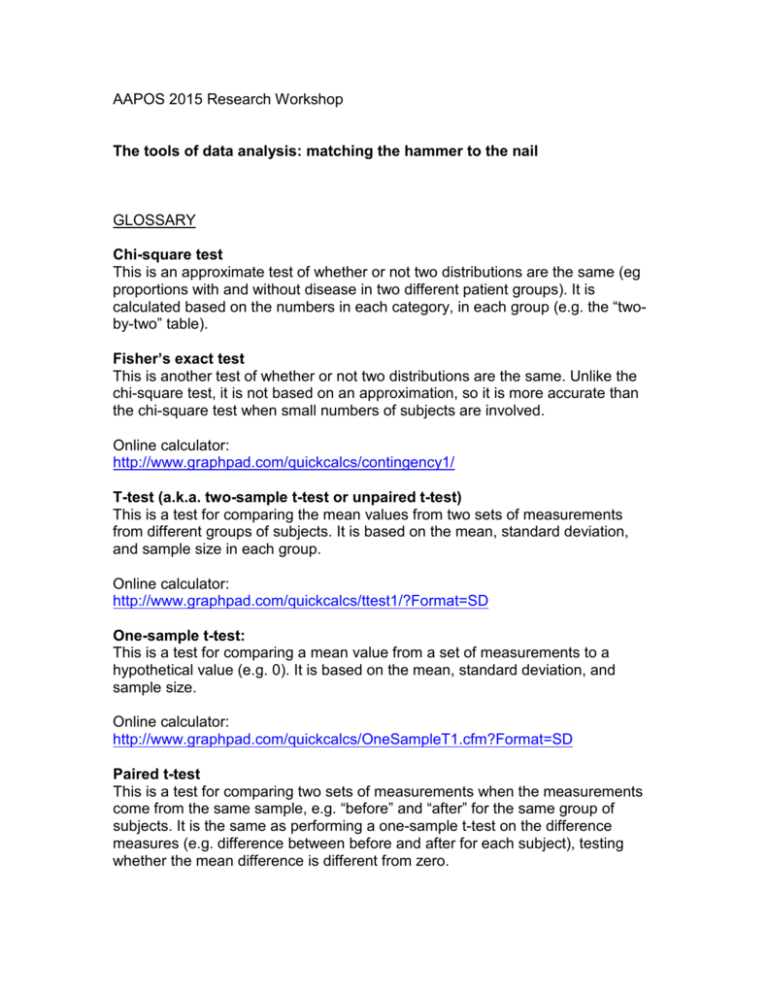
AAPOS 2015 Research Workshop
The tools of data analysis: matching the hammer to the nail
GLOSSARY
Chi-square test
This is an approximate test of whether or not two distributions are the same (eg
proportions with and without disease in two different patient groups). It is
calculated based on the numbers in each category, in each group (e.g. the “twoby-two” table).
Fisher’s exact test
This is another test of whether or not two distributions are the same. Unlike the
chi-square test, it is not based on an approximation, so it is more accurate than
the chi-square test when small numbers of subjects are involved.
Online calculator:
http://www.graphpad.com/quickcalcs/contingency1/
T-test (a.k.a. two-sample t-test or unpaired t-test)
This is a test for comparing the mean values from two sets of measurements
from different groups of subjects. It is based on the mean, standard deviation,
and sample size in each group.
Online calculator:
http://www.graphpad.com/quickcalcs/ttest1/?Format=SD
One-sample t-test:
This is a test for comparing a mean value from a set of measurements to a
hypothetical value (e.g. 0). It is based on the mean, standard deviation, and
sample size.
Online calculator:
http://www.graphpad.com/quickcalcs/OneSampleT1.cfm?Format=SD
Paired t-test
This is a test for comparing two sets of measurements when the measurements
come from the same sample, e.g. “before” and “after” for the same group of
subjects. It is the same as performing a one-sample t-test on the difference
measures (e.g. difference between before and after for each subject), testing
whether the mean difference is different from zero.
Online calculator:
You can enter the pairs of measurements:
http://www.graphpad.com/quickcalcs/ttest1/?Format=50
Or, you can calculate the difference measure for each subject, and use a onesample t-test (see above).
Two-tailed test
A two-tailed test should be used in most cases, because the real difference (e.g.
between two groups with mean values A and B) could theoretically go either way
(A>B or B>A).
Standard deviation (s.d.)
This is a measure of the degree of scatter of values around the mean value.
Excel has a function (STDEV) to calculate it.
Sensitivity
The proportion of actual cases that test positive.
Specificity
The proportion of actual non-cases (normals) that test negative.
Positive predictive value (PPV)
The chance that a positive test value is really an actual case. PPV depends on a
combination of sensitivity, specificity, and the frequency of cases in the
population.
Negative predictive value (NPV)
The chance that a negative test value is really normal. NPV depends on a
combination of sensitivity, specificity, and the frequency of cases in the
population.
Receiver-operating characteristic (ROC) curve
A graphical representation of all the combinations of sensitivity and specificity
that you can have as you vary the cutoff for a test. It is plotted as sensitivity on
the y-axis, against (1-specificity) on the x-axis. The area under the ROC curve is
a measure of overall accuracy, with 1 being a perfect test, and 0.5 being a
worthless test.
Non-parametric test
A non-parametric test may be appropriate when more common tests are not, eg
when the distribution of values is very skewed (i.e. nowhere near a normal
distribution). There are non-parametric equivalents to more commonly used
tests; eg the Wilcoxon rank sum test may be more appropriate than a 2-sample ttest when a distribution is very skewed in one direction (just as the median may
be a more appropriate summary measure than the mean).
Pearson’s correlation coefficient R
This is a measure of the strength of the linear correlation between an
“independent” variable (x) and a “dependent” variable (y). It can vary from 1
(perfect positive linear relationship; y increasing as x increases) to -1 (perfect
negative relationship; y decreasing as x increases), with 0 indicating no
relationship at all (y is totally independent of x). Excel has a function (CORREL)
to calculate this. R does not tell you how much y changes for a given change in x
(that’s a different number, the slope; see below); R just tells you how tight the
relationship is.
Linear regression
This is a statistical technique that finds the best-fitting line modeling the
relationship between x and y. The equation describing the line can then be used
to predict a value of y if you know the value of x, or to describe how much y
changes for a given change in x (this is the “slope” of the equation). The “add
trendline” function in excel performs linear regression on scatter-plot data and
shows the fitted line. You can display the equation and the R-squared value; the
R-squared value is the square of Pearson’s correlation coefficient R.
Logistic regression
Logistic regression is a form of linear regression, to be used when the dependent
(outcome) variable is a binary (e.g. yes/no) variable (rather than a continuous
variable). The logistic regression technique essentially first transforms the binary
variable to something that can be treated as a continuous variable, and then
performs ‘ordinary’ linear regression. It is very useful in data modeling when one
or more variables in the model are binary. Instead of y being a continuous
variable that changes with x, it is the frequency or probability of a “yes” vs. “no”
outcome that changes with x. The output of the equation is a value somewhere
between 0 and 1, representing the risk or probability of a yes vs. no outcome.
More details:
http://www.biostathandbook.com/simplelogistic.html
http://www.medcalc.org/manual/logistic_regression.php
Odds ratio (OR)
The odds ratio (OR) indicates the strength of the association between two
variables, classically termed “exposure” (think: treated/untreated; with/without the
gene; onset before/after a given age) and “outcome” (think: cured/not cured,
misaligned/straight, acuity above/below a given value). If OR>1, exposure is
associated with higher odds of outcome; if OR<1, exposure is associated with
lower odd of outcome. But, if the 95%-confidence interval (CI; see below)
includes the value 1, i.e., runs from a value below 1 to a value above 1, then the
OR is not significantly different from 1, and the exposure is not associated with
the odds of outcome.
Online calculator:
http://www.medcalc.org/calc/odds_ratio.php
Confidence interval (CI)
A sample that you study provides an estimate of a true value (e.g. an odds ratio,
or a prevalence). The 95% CI gives a range of values around this estimate;
chances are that the true value lies within this range.
Multiple or multivariate linear regression
This is linear regression, in which y is modeled as a function of a combination of
different x variables instead of just one x variable. This statistical technique
models the relationship between a dependent variable (e.g., y) and multiple
independent or explanatory variables (=x1 +x2 +x3, etc.) that each influence y.
The data set of x values and y values is used to create an equation that
describes that relationship. The equation can then be used to predict a value of y
for any subject if you know the values of x1, x2, x3, etc. The equation describes
how much y varies for a given change in x1 or x2 or x3 (each of which can have
a different “slope” or effect on y).
Multiple or multivariate logistic regression
This is logistic regression, in which the binary (yes/no) outcome y is modeled as
a function of a combination of different x variables instead of just one x variable.
The output of the equation is a value somewhere between 0 and 1, i.e., the risk
or probability that the outcome will be yes vs. no based upon the values of the
different x variables. The equation can be used to develop a prediction model
and predict an outcome for a given patient. The model also provides an odds
ratio for each different x variable, which describe the strength of the association
between each exposure (x variable) and the outcome (y).
Because these regression methods are “multivariate” or have multiple exposure
variables, they allow us to control for potential confounding variables in order to
determine if an association between a specific exposure or treatment (e.g., high
oxygen) and an outcome (e.g., severe ROP) exists independently when you
control for other factors (e.g., birth weight and gestational age).
Bland-Altman plot
A plot of data from two sets of measurements on the same samples/subjects,
where the difference between measure A and measure B is plotted against the
average of measure A and measure B for each pair of measurements (each
sample/subject).
Repeatability index
This is a measure of repeatability. It is 1.96 times the s.d. of the difference
between measure A and measure B.
Power Vector
To quantitatively analyze astigmatism in both magnitude and axis, we transform
clinical refractive error into a power vector notation consisting of (J0, J45, M).
This is a simple tool for astigmatism research, allowing averaging and
comparison of astigmatic refractive errors of different axes.
M
M is the same as the spherical equivalent refractive error.
J0
For sphero-cylindrical notation S + C axis A in degrees,
J0= (- C/2) * cos (2 * A)
J45
For sphero-cylindrical notation S + C axis A in degrees,
J45= (- C/2) * sin (2 * A)
Examples:
Sphero-cylindrical notation
J0
J45
Plus cylinder 1D axis 090
0.5
0
Plus cylinder 1D axis 180
-0.5
0
Plus cylinder 1D axis 045
0
-0.5
Plus cylinder 1D axis 135
0
0.5
Oblique astigmatism that is not exactly at axis 045 or 135 has
non-zero values for both J0 and J45 components.
LogMAR
LogMAR notation of visual acuity (VA) expresses VA in a form that is more
appropriate for mathematical manipulation (such as averaging) than Snellen
fraction or decimal notation. For VA represented as a fraction (such as x/20),
LogMAR VA = -(log (x/20)).
Examples:
LogMAR VA
0
0.1
0.2
0.3
Snellen VA
20/20
20/25
20/32
20/40