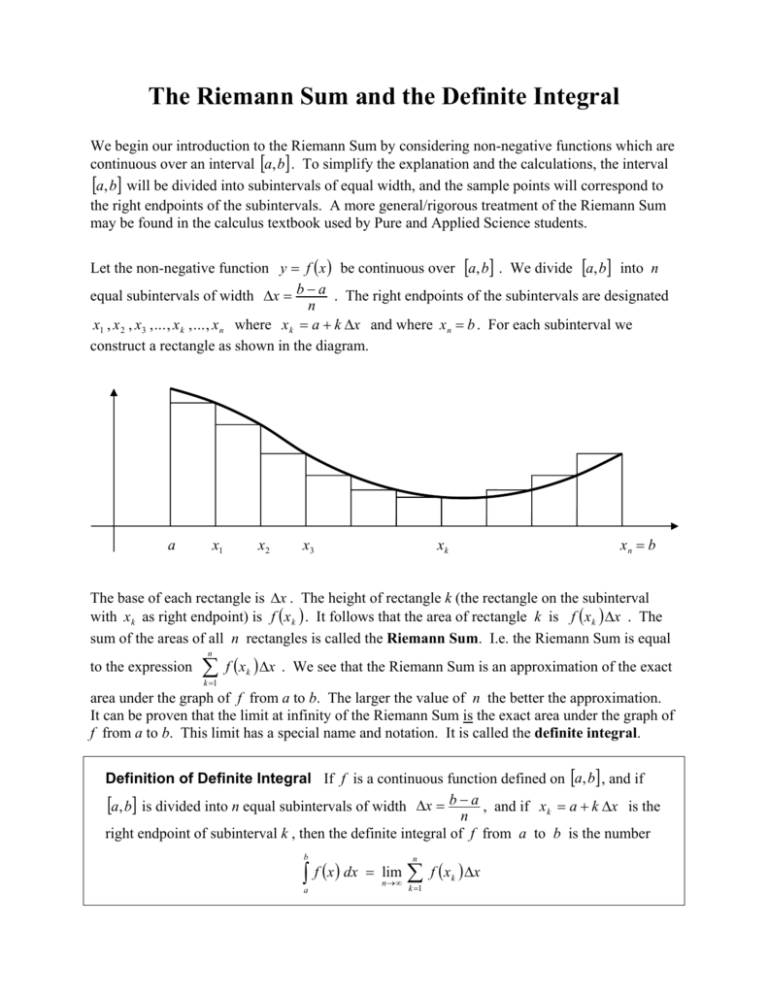
The Riemann Sum and the Definite Integral
We begin our introduction to the Riemann Sum by considering non-negative functions which are
continuous over an interval [a, b] . To simplify the explanation and the calculations, the interval
[a, b] will be divided into subintervals of equal width, and the sample points will correspond to
the right endpoints of the subintervals. A more general/rigorous treatment of the Riemann Sum
may be found in the calculus textbook used by Pure and Applied Science students.
Let the non-negative function y = f ( x ) be continuous over [a, b] . We divide [a, b] into n
equal subintervals of width ∆x = b − a . The right endpoints of the subintervals are designated
n
x1 , x 2 , x3 , ... , x k , ... , x n where x k = a + k ∆x and where x n = b . For each subinterval we
construct a rectangle as shown in the diagram.
a
x1
x2
x3
xn = b
xk
The base of each rectangle is ∆x . The height of rectangle k (the rectangle on the subinterval
with x k as right endpoint) is f ( x k ) . It follows that the area of rectangle k is f ( x k ) ∆x . The
sum of the areas of all n rectangles is called the Riemann Sum. I.e. the Riemann Sum is equal
n
to the expression
∑ f (x ) ∆x .
k =1
k
We see that the Riemann Sum is an approximation of the exact
area under the graph of f from a to b. The larger the value of n the better the approximation.
It can be proven that the limit at infinity of the Riemann Sum is the exact area under the graph of
f from a to b. This limit has a special name and notation. It is called the definite integral.
Definition of Definite Integral If f is a continuous function defined on [a, b] , and if
[a, b] is divided into n equal subintervals of width ∆x = b −n a , and if xk = a + k ∆x is the
right endpoint of subinterval k , then the definite integral of f from a to b is the number
b
∫
a
f ( x ) dx = lim
n→∞
n
∑ f ( x ) ∆x
k =1
k
Note: In the following two examples we consider non-negative functions on the interval [a, b] .
As explained last page, in such cases the definite integral from a to b is the area under the
curve from a to b (i.e. the area between the curve and the x-axis). The summation formulas in
the appendix will be needed in the solutions of these examples.
∫ (2 x
)
4
Example 1
Use the definition of definite integral to evaluate
2
+ 3 dx .
0
4
We subdivide the interval [ 0, 4] into n equal subintervals of width ∆x = 4 − 0 = .
n
n
2
32 k 2
4k
4
⎛ 4k ⎞
Then x k = 0 + k ⋅ =
+3 .
and
f (xk ) = 2 ⎜
⎟ + 3 → f (xk ) =
n
n
n2
⎝ n ⎠
⎞⎛ 4 ⎞
⎛ 32 k 2
128 k 2 12
f ( x k ) ∆x = ⎜⎜ 2 + 3 ⎟⎟ ⎜ ⎟ =
+
n
n3
⎠⎝ n ⎠
⎝ n
n
n
⎛ 128 k 2 12 ⎞
12
128 n 2
12 n
128 n (n + 1)(2n + 1)
⎟
⎜
(
)
f
x
x
=
k
+
=
⋅
+
⋅n
1
∆
=
+
∑
∑
∑
∑
k
3
3
3
⎟
⎜ n
n⎠
n k =1
n
6
n k =1
n
k =1
k =1 ⎝
128 ⎛ n ⎞ ⎛ n + 1 ⎞ ⎛ 2n + 1 ⎞
64 ⎛ 1 ⎞ ⎛
1⎞
⎟⎜
⎟ + 12 =
⎜1 + ⎟ ⎜ 2 + ⎟ + 12
⎜ ⎟⎜
6 ⎝ n ⎠⎝ n ⎠⎝ n ⎠
3 ⎝ n ⎠⎝
n⎠
=
∫ (2 x
4
0
2
n
⎡ 64 ⎛ 1 ⎞ ⎛
⎤
1⎞
+ 3 dx = lim ∑ f ( x k ) ∆x = lim ⎢ ⎜1 + ⎟ ⎜ 2 + ⎟ + 12⎥ = 64 (1)(2 ) + 12 = 164
n →∞
n →∞
3
3
n⎠
k =1
⎣ 3 ⎝ n ⎠⎝
⎦
)
∫ (8x − x ) dx .
5
Example 2
Use the definition of definite integral to evaluate
2
2
5− 2 3
= .
n
n
2
2
9k
12 k
⎛ 3k ⎞ ⎛ 3k ⎞
+ 12 .
f (xk ) = 8 ⎜ 2 + ⎟ − ⎜ 2 + ⎟ = − 2 +
n ⎠ ⎝
n ⎠
n
n
⎝
27 k 2 36 k 36
= − 3 + 2 +
n
n
n
We subdivide the interval [2 , 5] into n equal subintervals of width ∆x =
Then x k = 2 + k ⋅
3k
3
= 2+
n
n
and
⎞⎛ 3 ⎞
⎛ 9 k 2 12 k
f ( x k ) ∆x = ⎜⎜ − 2 +
+ 12 ⎟⎟ ⎜ ⎟
n
⎠⎝ n ⎠
⎝ n
2
n
n
⎛ 27 k
36 k 36 ⎞
27 n
36 n
36 n
f ( x k ) ∆x = ∑ ⎜⎜ − 3 + 2 + ⎟⎟ = − 3 ∑ k 2 + 2 ∑ k +
∑
∑1
n ⎠
n k =1
n
n
n k =1
n k =1
k =1
k =1 ⎝
= −
27 n (n + 1)(2n + 1)
36 n (n + 1)
36
9 ⎛ 1 ⎞⎛
1⎞
⎛ 1⎞
⋅
+ 2⋅
+
⋅ n = − ⎜1 + ⎟ ⎜ 2 + ⎟ + 18 ⎜1 + ⎟ + 36
3
6
2
2 ⎝ n ⎠⎝
n
n⎠
n
n
⎝ n⎠
∫ (8x − x ) dx
5
2
2
⎡ 9 ⎛ 1 ⎞⎛
⎤
1⎞
9
⎛ 1⎞
= lim ⎢− ⎜1 + ⎟ ⎜ 2 + ⎟ + 18 ⎜1 + ⎟ + 36⎥ = − (1)(2) + 18 (1) + 36 = 45
n →∞
n⎠
2
⎝ n⎠
⎣ 2 ⎝ n ⎠⎝
⎦
Page 2 of 7
Until now we have only considered non-negative functions on the interval [a, b] . In what
follows, the function may be negative on part, or all, of the interval. In those intervals where the
function is negative, the value of the Riemann Sum is the negative of the area between the curve
and the x-axis. It follows that the Riemann Sum may be a negative number.
EXERCISES Use the definition of definite integral (Riemann Sum) to evaluate each of the
following definite integrals. NOTE: these functions are not necessarily non-negative.
Nevertheless, the definition (Riemann Sum) may still be applied (as shown in the solutions).
5
1.
∫
2.
0
∫ (− 3x
2
+ 5 x − 1) dx
∫ (3x
+ 2 x dx
5.
2
)
2
)
+ 3 x + 5 dx
dx
6.
−5
∫ (4 x
2
)
− 5 x − 1 dx
∫
0
∫ (4 − 2 x ) dx
2
−8
∫ (1− 5x ) dx
2
2
12.
−2
5k
5
→ xk =
and f ( x k ) =
n
n
100 k
⎛ 20 k ⎞ ⎛ 5 ⎞
f ( x k ) ∆x = ⎜
⎟⎜ ⎟ =
n2
⎝ n ⎠⎝ n ⎠
n
n
100 n
⎛ 100 k ⎞
(
)
∆
=
=
f
x
x
⎜
⎟
∑
∑
∑k
k
2
n 2 k =1
⎠
k =1
k =1 ⎝ n
5
2
−3
9.
SOLUTIONS
1. ∆x =
∫ (x − 4 x ) dx
1
3
11.
)
− 2 x dx
5
2
−3
−1
2
0
0
8.
−2
∫ (x
∫ 2x
∫ (5 x
3
3.
4
0
10.
)
+ 10 dx
6
0
7.
2
0
4
4.
∫ (x
2
4 x dx
20 k
⎛ 5k ⎞
4 ⎜ ⎟ → f (xk ) =
n
⎝ n ⎠
=
100 ⎛ 1 ⎞
⎜1 + ⎟
2 ⎝ n⎠
n
⎡ ⎛ 1 ⎞⎤
4 x dx = lim ∑ f ( x k ) ∆x = lim ⎢50 ⎜1 + ⎟⎥ = 50
n →∞
n→∞
k =1
⎣ ⎝ n ⎠⎦
Page 3 of 7
∫x
−1
3
dx
2. ∆x =
2k
2
→ xk =
n
n
2
and
4k2
⎛ 2k ⎞
(
)
f (xk ) = ⎜
+
10
→
f
x
=
+ 10
⎟
k
n2
⎝ n ⎠
⎞⎛ 2 ⎞
⎛ 4k2
8 k 2 20
f ( x k ) ∆x = ⎜⎜ 2 + 10 ⎟⎟ ⎜ ⎟ = 3 +
n
n
⎠⎝ n ⎠
⎝ n
n
n
⎛ 8 k 2 20 ⎞
8 n 2 20 n
8 ⎛ 1 ⎞⎛
1⎞
⎟
⎜
(
)
=
∆
=
+
1 = ⎜1 + ⎟⎜ 2 + ⎟ + 20
f
x
x
k +
∑
∑
∑
k
3 ∑
⎟
⎜ n3
6 ⎝ n ⎠⎝
n ⎠
n k =1
n⎠
n k =1
k =1
k =1 ⎝
∫ (x
2
0
2
n
⎤
⎡ 4 ⎛ 1 ⎞⎛
1⎞
4
+ 10 ) dx = lim ∑ f (x k ) ∆x = lim ⎢ ⎜1 + ⎟⎜ 2 + ⎟ + 20⎥ = (1)(2 ) + 20 = 68
n →∞
n →∞ 3
3
3
n⎠
k =1
⎦
⎣ ⎝ n ⎠⎝
2
45 k 2 6 k
⎛ 3k ⎞
⎛ 3k ⎞
and f ( x k ) = 5 ⎜ ⎟ − 2⎜ ⎟ → f ( x k ) =
−
n
n2
⎝ n ⎠
⎝ n ⎠
⎛ 45 k 2 6 k ⎞ ⎛ 3 ⎞
135 k 2 18 k
⎟⎟ ⎜ ⎟ =
f ( x k ) ∆x = ⎜⎜ 2 −
− 2
n ⎠⎝ n ⎠
n3
n
⎝ n
n
135 n 2 18 n
135 ⎛ 1 ⎞⎛
1 ⎞ 18 ⎛ 1 ⎞
(
)
∆
=
f
x
x
k − 2∑k =
⎜1 + ⎟⎜ 2 + ⎟ − ⎜1 + ⎟
∑
k
3 ∑
6 ⎝ n ⎠⎝
n⎠ 2 ⎝ n⎠
n k =1
n k =1
k =1
3
⎡ 45 ⎛ 1 ⎞ ⎛
1⎞
45
⎛ 1 ⎞⎤
2
(1)(2) − 9 (1) = 36
⎜1 + ⎟ ⎜ 2 + ⎟ − 9 ⎜1 + ⎟ ⎥ =
⎢
∫0 (5 x − 2 x ) dx = lim
n →∞
2
n⎠
⎝ n ⎠⎦
⎣ 2 ⎝ n ⎠⎝
3k
3
3. ∆x =
→ xk =
n
n
4k
4
4. ∆x =
→ xk =
n
n
and
f (xk ) =
2
48 k 2 20 k
⎛ 4k ⎞
⎛ 4k ⎞
− 3⎜
−1
⎟ + 5⎜
⎟ − 1 → f (x k ) = − 2 +
n
n
⎝ n ⎠
⎝ n ⎠
192 k 2 80 k 4
= −
+ 2 −
n
n3
n
⎛ 48 k 2 20 k ⎞ ⎛ 4 ⎞
f ( x k ) ∆x = ⎜⎜ − 2 +
− 1⎟⎟ ⎜ ⎟
n
n
⎠⎝ n ⎠
⎝
n
n
192
80 n
4 n
192 ⎛ 1 ⎞⎛
1 ⎞ 80 ⎛ 1 ⎞
2
f ( x k ) ∆x = − 3 ∑ k + 2 ∑ k − ∑ 1 = −
⎜1 + ⎟⎜ 2 + ⎟ + ⎜1 + ⎟ − 4
∑
6 ⎝ n ⎠⎝
n i =1
n⎠ 2 ⎝ n⎠
n i =1
n i =1
i =1
∫ (− 3x
4
0
2
⎡
1⎞
⎛ 1 ⎞⎛
⎛ 1⎞ ⎤
+ 5 x − 1 dx = lim ⎢− 32 ⎜1 + ⎟⎜ 2 + ⎟ + 40 ⎜1 + ⎟ − 4⎥ = − 32 (1)(2 ) + 40 (1) − 4 = − 28
n →∞
n⎠
⎝ n ⎠⎝
⎝ n⎠ ⎦
⎣
)
2
2k ⎞
8 k 2 32 k
⎛
and f ( x k ) = 2 ⎜ 4 +
+ 32
⎟ → f (x k ) = 2 +
n ⎠
n
n
⎝
⎞⎛ 2 ⎞
⎛ 8 k 2 32 k
16 k 2 64 k 64
f ( x k ) ∆x = ⎜⎜ 2 +
+ 32 ⎟⎟ ⎜ ⎟ =
+ 2 +
n
n
n3
n
⎠⎝ n ⎠
⎝ n
n
16 n 2
64 n
64 n
16 ⎛ 1 ⎞⎛
1 ⎞ 64 ⎛ 1 ⎞
(
)
∆
=
+
+
1 =
f
x
x
k
k
⎜1 + ⎟⎜ 2 + ⎟ − ⎜1 + ⎟ + 64
∑
∑
k
3 ∑
2 ∑
6 ⎝ n ⎠⎝
n i =1
n⎠ 2 ⎝ n⎠
n i =1
n i =1
i =1
6
⎡8 ⎛ 1 ⎞ ⎛
1⎞
8
304
⎛ 1 ⎞⎤
2
1 + ⎟ ⎜ 2 + ⎟ + 64 ⎜1 + ⎟⎥ = (1)(2) + 32 (1) + 64 =
⎜
⎢
∫4 2 x dx = lim
n →∞ 3
3
n⎠
3
⎝ n ⎠⎦
⎣ ⎝ n ⎠⎝
2k
2
5. ∆x =
→ xk = 4 +
n
n
Page 4 of 7
2
4k
64 k 2 28 k
4
⎛ 4k ⎞
⎛ 4k ⎞
(
)
and f ( x k ) = ⎜1 +
4
1
→
=
−
−
−3
−
+
→ xk = 1+
f
x
⎜
⎟
⎟
k
n
n
n ⎠
n ⎠
n
n2
⎝
⎝
⎞⎛ 4 ⎞
⎛ 64 k 2 28 k
256 k 2 112 k 12
f ( x k ) ∆x = ⎜⎜ − 2 −
− 3 ⎟⎟ ⎜ ⎟ = −
− 2 −
3
n
n
n
n
n
n
⎝
⎠
⎠
⎝
6. ∆x =
n
∑
k =1
f ( x k ) ∆x = −
256 n 2 112 n
12 n
256 ⎛ 1 ⎞⎛
1 ⎞ 112 ⎛ 1 ⎞
−
−
1= −
k
k
⎜1 + ⎟⎜ 2 + ⎟ −
⎜1 + ⎟ − 12
∑
3 ∑
2 ∑
6 ⎝ n ⎠⎝
n k =1
n⎠ 2 ⎝ n⎠
n k =1
n k =1
⎡ 128 ⎛ 1 ⎞⎛
⎤
1⎞
128
460
⎛ 1⎞
∫ (x − 4 x )dx = lim ⎢⎣− 3 ⎜⎝1+ n ⎟⎠⎜⎝ 2 + n ⎟⎠ − 56 ⎜⎝1+ n ⎟⎠ − 12⎥⎦ = − 3 (1)(2) − 56 (1) − 12 = − 3
5
2
n →∞
1
2
2k
12 k 2 20 k
2
⎞
⎛ 2k
⎞
⎛ 2k
→ xk =
− 2 and f ( x k ) = 3 ⎜
− 2⎟ + 2⎜
− 2 ⎟ → f (xk ) = 2 −
+8
n
n
n
n
⎝ n
⎠
⎝ n
⎠
⎞⎛ 2 ⎞
⎛ 12 k 2 20 k
24 k 2 40 k 16
f ( x k ) ∆x = ⎜⎜ 2 −
+ 8 ⎟⎟ ⎜ ⎟ =
− 2 +
3
n
n
n
n
n
n
⎝
⎠
⎠
⎝
7. ∆x =
n
∑
k =1
f ( x k ) ∆x =
∫ (3x
0
2
−2
24 n 2
40 n
16 n
24 ⎛ 1 ⎞⎛
1 ⎞ 40 ⎛ 1 ⎞
−
+
1 =
k
k
⎜1 + ⎟⎜ 2 + ⎟ − ⎜1 + ⎟ + 16
∑
3 ∑
2 ∑
6 ⎝ n ⎠⎝
n k =1
n⎠ 2 ⎝ n⎠
n k =1
n k =1
⎡ ⎛ 1 ⎞⎛
⎤
1⎞
⎛ 1⎞
+ 2 x ) dx = lim ⎢4 ⎜1 + ⎟⎜ 2 + ⎟ − 20 ⎜1 + ⎟ + 16⎥ = 4 (1)(2) − 20(1) + 16 = 4
n →∞
n⎠
⎝ n⎠
⎣ ⎝ n ⎠⎝
⎦
2
3k
36 k 2 87 k
3
⎛ 3k
⎞
⎛ 3k
⎞
→ xk =
− 3 and f ( x k ) = 4 ⎜
− 3⎟ − 5 ⎜
− 3 ⎟ − 1 → f (xk ) = 2 −
+ 50
n
n
n
n
⎠
⎝ n
⎠
⎝ n
⎞⎛ 3 ⎞
⎛ 36 k 2 87 k
108 k 2 261 k 150
f ( x k ) ∆x = ⎜⎜ 2 −
+ 50 ⎟⎟ ⎜ ⎟ =
− 2 +
n
n
n3
n
⎠⎝ n ⎠
⎝ n
8. ∆x =
108 n 2
261 n
150 n
108 ⎛ 1 ⎞⎛
1 ⎞ 261 ⎛ 1 ⎞
−
+
1 =
k
k
⎜1 + ⎟⎜ 2 + ⎟ −
⎜1 + ⎟ + 150
∑
∑
3 ∑
2 ∑
6 ⎝ n ⎠⎝
n k =1
n⎠ 2 ⎝ n⎠
n k =1
n k =1
k =1
0
⎡ ⎛ 1 ⎞⎛
⎤
1 ⎞ 261 ⎛ 1 ⎞
261
111
2
(
18 ⎜1 + ⎟⎜ 2 + ⎟ −
1 + ⎟ + 150⎥ = 18 (1)(2 ) −
1) + 150 =
⎜
⎢
∫−3(4 x − 5 x −1)dx = lim
n →∞
2
n⎠ 2 ⎝ n⎠
2
⎣ ⎝ n ⎠⎝
⎦
n
f ( x k ) ∆x =
2
5k
50 k 2 160 k
5
⎛ 5k
⎞
9. ∆x =
→ xk =
− 8 and f ( x k ) = 4 − 2 ⎜
− 8 ⎟ → f (xk ) = − 2 +
− 124
n
n
n
n
⎝ n
⎠
⎞⎛ 5 ⎞
⎛ 50 k 2 160 k
250 k 2 800 k 620
⎟
⎜
f ( x k ) ∆x = ⎜ − 2 +
− 124 ⎟ ⎜ ⎟ = −
+ 2 −
n
n
n
n3
n
⎠⎝ n ⎠
⎝
n
n
250
∑ f (x ) ∆x = − n ∑ k
k
k =1
3
−3
k =1
2
+
800 n
620 n
250 ⎛ 1 ⎞⎛
1 ⎞ 800 ⎛ 1 ⎞
−
1= −
k
⎜1 + ⎟⎜ 2 + ⎟ +
⎜1 + ⎟ − 620
∑
∑
2
6 ⎝ n ⎠⎝
n k =1
n⎠ 2 ⎝ n⎠
n k =1
⎡ 125 ⎛ 1 ⎞ ⎛
1⎞
⎤
125
910
⎛ 1⎞
(1)( 2 ) + 400 (1) − 620 = −
⎜ 1 + ⎟ ⎜ 2 + ⎟ + 400 ⎜ 1 + ⎟ − 620 ⎥ = −
3 ⎝ n ⎠⎝
3
3
n⎠
⎝ n⎠
⎦
∫ ( 4 − 2 x ) dx = lim ⎢⎣ −
2
−8
n →∞
Page 5 of 7
2
4k
16 k 2 28 k
4
⎛ 4k
⎞
⎛ 4k
⎞
− 5 ⎟ + 5 → f (xk ) = 2 −
→ xk =
− 5 and f ( x k ) = ⎜
− 5⎟ + 3⎜
+ 15
n
n
n
n
⎝ n
⎠
⎝ n
⎠
⎞⎛ 4 ⎞
⎛ 16 k 2 28 k
64 k 2 112 k 60
f ( x k ) ∆x = ⎜⎜ 2 −
+ 15 ⎟⎟ ⎜ ⎟ =
− 2 +
3
n
n
n
n
n
n
⎝
⎠
⎠
⎝
10. ∆x =
n
∑
k =1
f ( x k ) ∆x =
−1
∫ (x
−5
2
64 n 2
112 n
60 n
32 ⎛ 1 ⎞⎛
1⎞
⎛ 1⎞
−
+
1 =
k
k
⎜1 + ⎟⎜ 2 + ⎟ − 56 ⎜1 + ⎟ + 60
∑
3 ∑
2 ∑
3 ⎝ n ⎠⎝
n k →1
n⎠
n k =1
n k =1
⎝ n⎠
⎡ 32 ⎛ 1 ⎞ ⎛
⎤
1⎞
32
⎛ 1⎞
(1)(2) − 56 (1) + 60 = 76
+ 3 x + 5 dx = lim ⎢ ⎜1 + ⎟ ⎜ 2 + ⎟ − 56 ⎜1 + ⎟ + 60⎥ =
n →∞
3
n⎠
3
⎝ n⎠
⎣ 3 ⎝ n ⎠⎝
⎦
)
2
125 k 2 100 k
⎛ 5k
⎞
and f ( x k ) = 1 − 5 ⎜
+
− 19
− 2 ⎟ → f (xk ) = −
n
n2
⎝ n
⎠
⎞⎛ 5 ⎞
⎛ 125 k 2 100 k
625 k 2 500k 95
⎟
f ( x k ) ∆x = ⎜⎜ −
19
+
−
=
−
+ 2 −
⎜
⎟
⎟ n
n
n
n2
n3
n
⎠⎝ ⎠
⎝
5k
5
11. ∆x =
→ xk =
−2
n
n
625 n 2 500 n
95 n
625 ⎛ 1 ⎞⎛
1 ⎞ 500 ⎛ 1 ⎞
+
−
1 = −
k
k
⎜1 + ⎟⎜ 2 + ⎟ +
⎜1 + ⎟ − 95
∑
∑
3 ∑
2 ∑
6 ⎝ n ⎠⎝
2 ⎝ n⎠
n k =1
n⎠
n k =1
n k =1
k =1
3
⎡ 625 ⎛ 1 ⎞⎛
⎤
1⎞
625
160
⎛ 1⎞
2
(
−
1 + ⎟⎜ 2 + ⎟ + 250 ⎜1 + ⎟ − 95⎥ = −
1)(2 ) + 250 (1) − 95 = −
⎜
⎢
∫−2 1 − 5x dx = lim
n →∞
6
n⎠
3
⎝ n⎠
⎣ 6 ⎝ n ⎠⎝
⎦
n
(
f ( x k ) ∆x = −
)
3k
3
12. ∆x =
→ xk =
−1
n
n
and
⎛ 3k ⎞
− 1⎟
f (xk ) = ⎜
⎝ n
⎠
3
→
f (x k ) =
27 k 3 27 k 2 9 k
− 2 +
−1
n
n3
n
⎞⎛ 3 ⎞
⎛ 27 k 3 27 k 2 9 k
81k 3 81 k 2 27 k 3
⎟
⎜
= ⎜ 3 − 2 +
− 1⎟ ⎜ ⎟ =
− 3 + 2 −
n
n
n4
n
n
n
⎠⎝ n ⎠
⎝ n
n
⎛ 81k 3 81 k 2 27 k 3 ⎞
81 n
81 n
27 n
3 n
f ( xk ) ∆x = ∑ ⎜ 4 − 3 + 2 − ⎟ = 4 ∑ k 3 − 3 ∑ k 2 + 2 ∑ k − ∑ 1
n⎠
n k =1
n
n
n k =1
n k =1
n k =1
k =1 ⎝ n
f ( x k ) ∆x
n
∑
k =1
3
27 n (n + 1)
81 n (n + 1)(2n + 1)
81 n 2 (n + 1)
= 4⋅
− 3⋅
+ 2⋅
− ⋅n
n
2
6
4
n
n
n
2
81 ⎛ 1 ⎞
27 ⎛ 1 ⎞ ⎛
1⎞
27 ⎛ 1 ⎞
=
⎜1 + ⎟ −
⎜1 + ⎟ ⎜ 2 + ⎟ +
⎜1 + ⎟ − 3
n⎠
4 ⎝ n⎠
2 ⎝ n ⎠⎝
2 ⎝ n⎠
2
⎡ 81 ⎛ 1 ⎞ 2 27 ⎛ 1 ⎞ ⎛
⎤
1 ⎞ 27 ⎛ 1 ⎞
3
lim
1
=
+
−
+
+
+
+
−
1
2
1
3
x
dx
⎜
⎟
⎜
⎟
⎜
⎟
⎜
⎟
⎢
⎥
∫
n →∞ 4
2 ⎝ n ⎠⎝
2 ⎝ n⎠
n⎠
−1
⎣⎢ ⎝ n ⎠
⎦⎥
2
27
⎡ 81 2 27
(1) − 3⎤⎥ = 15
= ⎢ (1) − (1)(2) +
2
2
4
⎣4
⎦
Page 6 of 7
APPENDIX
The following are useful formulas for working with summation notation.
n
1.
∑c
= nc
k =1
n
2.
∑
k =1
n
c ak = c ∑ ak
k =1
n
3.
∑ ( ak + bk )
n
∑
=
k =1
n
4.
∑ ( ak − bk )
k =1
n
5.
∑k
n
∑k
k =1
∑
k =1
ak −
∑b
k
k =1
n
∑b
k =1
k
n (n + 1)(2n + 1)
6
=
3
n 2 (n + 1)
=
4
n
∑k
n
2
k =1
7.
=
n
n (n + 1)
2
=
k =1
6.
k =1
ak +
2
Page 7 of 7