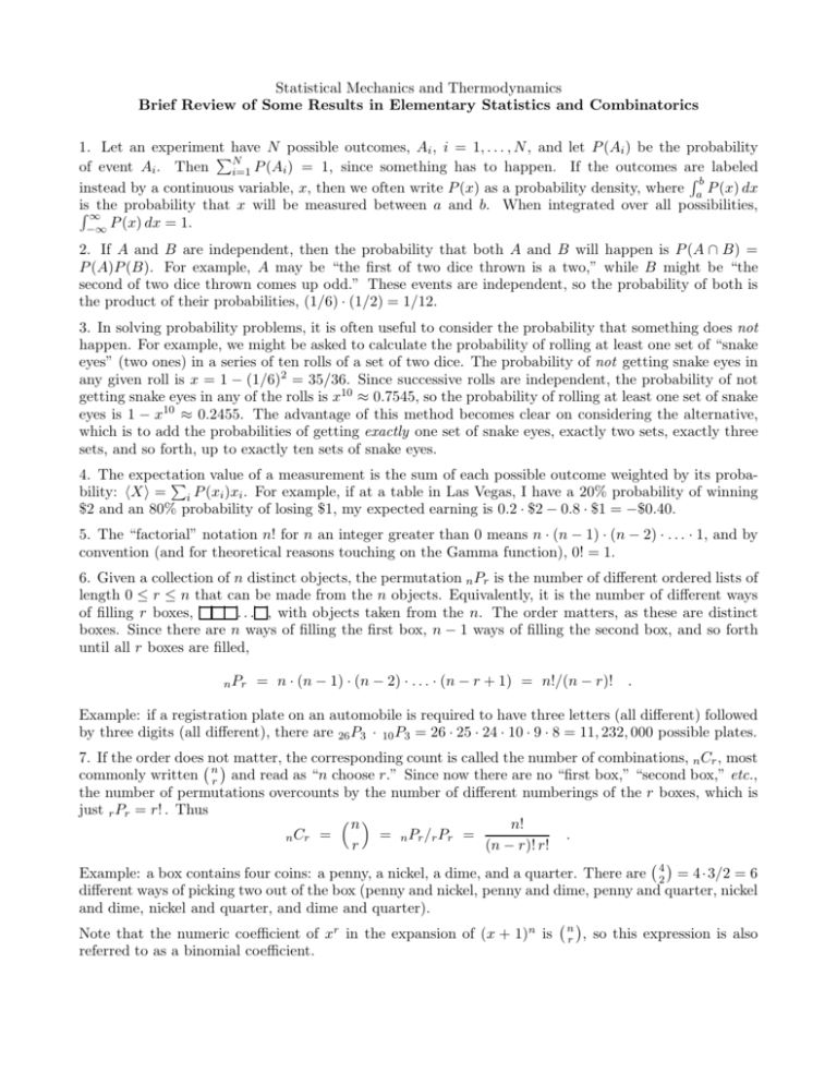
Statistical Mechanics and Thermodynamics
Brief Review of Some Results in Elementary Statistics and Combinatorics
1. Let an experiment have N possible outcomes, Ai , i = 1, . . . , N , and let P (Ai ) be the probability
PN
of event Ai . Then
labeled
i=1 P (Ai ) = 1, since something has to happen. If the outcomes are
Rb
instead by a continuous variable, x, then we often write P (x) as a probability density, where a P (x) dx
is
R ∞the probability that x will be measured between a and b. When integrated over all possibilities,
−∞ P (x) dx = 1.
2. If A and B are independent, then the probability that both A and B will happen is P (A ∩ B) =
P (A)P (B). For example, A may be “the first of two dice thrown is a two,” while B might be “the
second of two dice thrown comes up odd.” These events are independent, so the probability of both is
the product of their probabilities, (1/6) · (1/2) = 1/12.
3. In solving probability problems, it is often useful to consider the probability that something does not
happen. For example, we might be asked to calculate the probability of rolling at least one set of “snake
eyes” (two ones) in a series of ten rolls of a set of two dice. The probability of not getting snake eyes in
any given roll is x = 1 − (1/6)2 = 35/36. Since successive rolls are independent, the probability of not
getting snake eyes in any of the rolls is x10 ≈ 0.7545, so the probability of rolling at least one set of snake
eyes is 1 − x10 ≈ 0.2455. The advantage of this method becomes clear on considering the alternative,
which is to add the probabilities of getting exactly one set of snake eyes, exactly two sets, exactly three
sets, and so forth, up to exactly ten sets of snake eyes.
4. The expectation
value of a measurement is the sum of each possible outcome weighted by its probaP
bility: hXi = i P (xi )xi . For example, if at a table in Las Vegas, I have a 20% probability of winning
$2 and an 80% probability of losing $1, my expected earning is 0.2 · $2 − 0.8 · $1 = −$0.40.
5. The “factorial” notation n! for n an integer greater than 0 means n · (n − 1) · (n − 2) · . . . · 1, and by
convention (and for theoretical reasons touching on the Gamma function), 0! = 1.
6. Given a collection of n distinct objects, the permutation n Pr is the number of different ordered lists of
length 0 ≤ r ≤ n that can be made from the n objects. Equivalently, it is the number of different ways
of filling r boxes,
. . . , with objects taken from the n. The order matters, as these are distinct
boxes. Since there are n ways of filling the first box, n − 1 ways of filling the second box, and so forth
until all r boxes are filled,
n Pr
= n · (n − 1) · (n − 2) · . . . · (n − r + 1) = n!/(n − r)! .
Example: if a registration plate on an automobile is required to have three letters (all different) followed
by three digits (all different), there are 26 P3 · 10 P3 = 26 · 25 · 24 · 10 · 9 · 8 = 11, 232, 000 possible plates.
7. If the order does not
matter, the corresponding count is called the number of combinations, n Cr , most
commonly written nr and read as “n choose r.” Since now there are no “first box,” “second box,” etc.,
the number of permutations overcounts by the number of different numberings of the r boxes, which is
just r Pr = r! . Thus
n
n!
= n Pr /r Pr =
.
n Cr =
r
(n − r)! r!
Example: a box contains four coins: a penny, a nickel, a dime, and a quarter. There are 42 = 4 · 3/2 = 6
different ways of picking two out of the box (penny and nickel, penny and dime, penny and quarter, nickel
and dime, nickel and quarter, and dime and quarter).
Note that the numeric coefficient of xr in the expansion of (x + 1)n is nr , so this expression is also
referred to as a binomial coefficient.