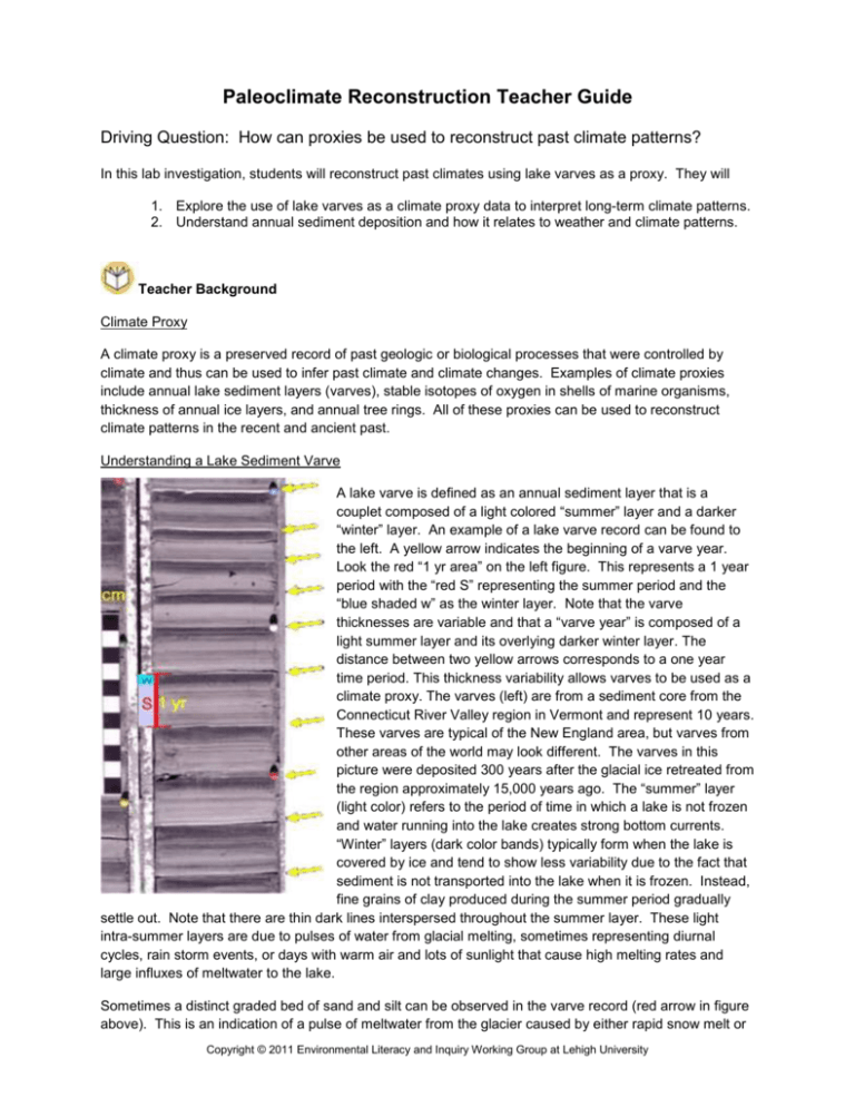
Paleoclimate Reconstruction Teacher Guide
Driving Question: How can proxies be used to reconstruct past climate patterns?
In this lab investigation, students will reconstruct past climates using lake varves as a proxy. They will
1. Explore the use of lake varves as a climate proxy data to interpret long-term climate patterns.
2. Understand annual sediment deposition and how it relates to weather and climate patterns.
Teacher Background
Climate Proxy
A climate proxy is a preserved record of past geologic or biological processes that were controlled by
climate and thus can be used to infer past climate and climate changes. Examples of climate proxies
include annual lake sediment layers (varves), stable isotopes of oxygen in shells of marine organisms,
thickness of annual ice layers, and annual tree rings. All of these proxies can be used to reconstruct
climate patterns in the recent and ancient past.
Understanding a Lake Sediment Varve
A lake varve is defined as an annual sediment layer that is a
couplet composed of a light colored “summer” layer and a darker
“winter” layer. An example of a lake varve record can be found to
the left. A yellow arrow indicates the beginning of a varve year.
Look the red “1 yr area” on the left figure. This represents a 1 year
period with the “red S” representing the summer period and the
“blue shaded w” as the winter layer. Note that the varve
thicknesses are variable and that a “varve year” is composed of a
light summer layer and its overlying darker winter layer. The
distance between two yellow arrows corresponds to a one year
time period. This thickness variability allows varves to be used as a
climate proxy. The varves (left) are from a sediment core from the
Connecticut River Valley region in Vermont and represent 10 years.
These varves are typical of the New England area, but varves from
other areas of the world may look different. The varves in this
picture were deposited 300 years after the glacial ice retreated from
the region approximately 15,000 years ago. The “summer” layer
(light color) refers to the period of time in which a lake is not frozen
and water running into the lake creates strong bottom currents.
“Winter” layers (dark color bands) typically form when the lake is
covered by ice and tend to show less variability due to the fact that
sediment is not transported into the lake when it is frozen. Instead,
fine grains of clay produced during the summer period gradually
settle out. Note that there are thin dark lines interspersed throughout the summer layer. These light
intra-summer layers are due to pulses of water from glacial melting, sometimes representing diurnal
cycles, rain storm events, or days with warm air and lots of sunlight that cause high melting rates and
large influxes of meltwater to the lake.
Sometimes a distinct graded bed of sand and silt can be observed in the varve record (red arrow in figure
above). This is an indication of a pulse of meltwater from the glacier caused by either rapid snow melt or
Copyright © 2011 Environmental Literacy and Inquiry Working Group at Lehigh University
Paleoclimate Reconstruction Teacher Guide
2
the sudden opening of sub-glacial tunnels. This is sometimes capped by a thin silty clay bed. It is
frequently the coarsest sediment deposited as part of the summer layer.
Changes in varve thickness are associated with changes in meltwater output and sediment deposition,
which varies with changes in the weather. For example a warmer year will have a thicker annual varve
layer resulting from more meltwater carrying sediment from the glacier. A colder year will have a
thinner annual varve layer. In most glacial varve environments, the summer season is shorter than the
winter season. However, in some locations, summer sediments may vary greatly (such as in the figure
above) depending on bedrock source and erosion rates.
In the classroom investigation, the varves were obtained from a sediment core that was taken in an
ancient glacial lake that was initially proximal (close) to the margin of a glacier and over time gradually
becomes distal (moved further away from the margin).
Varves as Records of Deglaciation
Varve chronology (using varves to set up a time scale) is a useful tool in deciphering the history of ice
retreat or deglaciation. Varves are capable of recording various deglaciation events in varve years, which
can then be calibrated using absolute dating techniques such as radiocarbon dating. Radiocarbon dating
is a method that utilizes
the decay of the
naturally occurring
carbon-14 isotope. It is
useful in dating organic
material that is less than
40,000 years old.
A deglaciation event
refers to the glacial ice
retreating and it can be
viewed in the
Northeastern United
States in the picture to
the right. The colored
lines mark different
landforms that were left
by the glacier as it
Bethlehem, PA
retreated. These are
most commonly known
as terminal or
recessional moraines. The numbers associated with each line refer to the number of years before
present (in thousands of years) that the glacier paused to develop that specific landform. As can be seen
by the picture, the margin of the glacier reached its furthest extent about ~28 thousand years ago (red
line) and then retreated northwards. Lakes that contain varves can be referred to as distal (far away) or
proximal (near) to the ice front. The black diamond indicates the location of the core used for this
classroom investigation. The red diamond indicates the location of Bethlehem, PA.
Copyright © 2011 Environmental Literacy and Inquiry Working Group at Lehigh University
Paleoclimate Reconstruction Teacher Guide
3
The Basics of Coring
Detailed surficial
mapping of ancient
glacial lakes can be
used to find lake
varve exposures.
Once a varve outcrop
is located it can be
cored and measured
to produce a varve
record. Varve
records can be
correlated and
assembled into a
regional composite
chronology to
understand the
spatial pattern of
climate change as
South
seen in the figure to
the right. The letters correspond to different sediment cores. Core
“A” was deposited in the southernmost location. Core “H” was
deposited in the northernmost location. The yellow “time” arrow is
used to show the relative time periods of each core. Core “A” is
older than Core “B”. Note the age of the basal varve gets younger
in the direction of the ice retreat (towards the north).
North
In 1882, geologists began to use varve chronology in Sweden. In
1920 measurements of varve thicknesses in the field were used in
America. This method is still used today; however it is
recommended that varves are measured in a lab from outcrop
cores. Cores allow for more careful measurement and provide
samples for doing other things with the sediment such as studying
microfossils.
In many places surface varve exposures of sufficient
depth to assemble varve sequences cannot be found. In
these areas deep drilling may be employed to recover
cores of varve sections. A hollow stem auger continuous
sampling system can allow the recovery of samples from
5-ft core drives. The sampling system is usually limited to
a depth of 120-200 feet depending on the resistance of
the material to the auger and the torque limitations of the
drilling truck. Taking small overlapping cores (2 feet) is
the ideal way to sample a varve section. Once back in
lab, the cores can be digitally imaged and then analyzed
for inter-annual varve thickness.
The core for this lab investigation was taken along Canoe
Brook in Dummerston, Vermont and represents a period
of time about 14,900-14,600 years ago. These varves
formed in glacial Lake Hitchcock in southern Vermont
Copyright © 2011 Environmental Literacy and Inquiry Working Group at Lehigh University
Paleoclimate Reconstruction Teacher Guide
4
which was somewhat proximal to the retreating glacier. The lake was named for Edward Hitchcock who
was a geologist from Amherst College that studied the lake. As can be seen from the paleoclimate
reconstruction key below, the climate is warmer (# 1) at the beginning of the varve record and then
transitions into a colder period (# 2). The climate record then indicates a period of alternating warm and
cold years (# 3). Beginning at varve year 5875 we see very thin varve sections. This is due to the fact
that the glacier was proximal to the lake at the beginning of the record and retreated away from the lake
as time moved towards the present. As the source of sediment retreats (glacier) the amount of sediment
being deposited each year decreases. This indicates a warmer climate.
#1) Warmer Years
#3) Alternating years of
warm and cold weather
#4) Retreating glacier (This is an
indication of a warm period). The
sediment supply has been cut off.
#2) Cooler Years
LAB OVERVIEW
In the student investigation, the data is divided into 10 core segments, each composed of about 30 varve
layers. Core 1 is split into two parts labeled “Core 1a” and “Core 1b”. Both parts should be combined and
plotted on the Core 1 graph (Varve Years 5685 to 5715). Varve measurements should be taken in tenths
of centimeters (millimeters) starting at the bottom of each core and working upwards. Measurements less
than 1 millimeter are recorded in the Measurement Table as 1mm and should be plotted and included on
the core graph. Five year increments are marked within each core to help the students stay organized.
Measurements should first be transferred to the Measurement Table on the core data handout and then
graphed once all of the data has been collected.
Copyright © 2011 Environmental Literacy and Inquiry Working Group at Lehigh University
Paleoclimate Reconstruction Teacher Guide
5
Important Notes: The original data set used in this lab has been scaled down by a factor of 10 to insure
that both the core and Measurement Table fit on a normal 8.5” x 11” page. Cool years and warm years
are determined relative to a particular location. In this learning activity for this particular location, cooler
years are indicated by varve thicknesses that are less than 1.5 cm. Warmer years are indicated by varve
thicknesses greater than 1.5 cm.





Materials Needed:
Paleoclimate Reconstruction Using Lake Varves PowerPoint
Paleoclimate Reconstruction Core Data Handout
Pencil
Ruler
Colored markers
Step 1: Present the Paleoclimate Reconstruction Using Lake Varves PowerPoint Slideshow
to the Students.
This PowerPoint slideshow is designed to provide your students with requisite background
information on the use of lake varves as a climate proxy. It also provides an overview of the lab
investigation’s core data and associated materials to help them understand how to measure and
graph the varve data.
Step 2: Distribute the Paleoclimate Reconstruction Laboratory Materials to the students.
a) Paleoclimate Reconstruction Investigation Guide
b) Paleoclimate Reconstruction Core Data Handout
There are 10 Core data sheets that are to be distributed to groups of students in the classroom. Students
can work individually or in groups of 2. Each of the 10 cores must be measured, recorded, and graphed in
order to analyze the entire paleoclimate record. In larger classes, you may wish to have students or
student groups complete multiple versions of each core and compare their results with each other as a
measurement validation check.
Important: Core 1 is split into two parts labeled “Core 1a” and “Core 1b”. Both parts need to be combined
together and plotted on the Core 1 graph (Varve Years 5685 to 5715).
Note: The data measurements for Core 5 are provided. The varve thicknesses for Core 5 are too small to
be measured accurately in the classroom. The Core 5 graph (Varve Years 5805 to 5834) will be used
later in the investigation during the analysis of the cumulative climate proxy record of all the combined
cores.
Step 3: Paleoclimate Reconstruction: Individual Cores
Instruct the students to measure the thickness of each varve layer in their core. Each varve year
corresponds to the distance between two line segments in a core. Students should record the
measurements in the associated Measurement Table beginning with the bottom of the core. An example
of Core 1 is shown below. Students should measure the thickness of each varve layer (# 1 below) and
than transfer that measurement to the corresponding year on the Measurement Table (# 2 below). New
England Varve year 5693 is used as an example.
Note: If the thickness of a varve is less than 0.1 cm, the answer has been pre-recorded in the
measurement table. Also, it is much easier to have students measure their cores by starting at the
bottom of the core (oldest and smaller year number) and work upwards (youngest and higher year
number).
Copyright © 2011 Environmental Literacy and Inquiry Working Group at Lehigh University
Paleoclimate Reconstruction Teacher Guide
6
After all core measurements have been recorded in the Measurement Table, instruct students to plot their
data on the core graph as shown below (#3 below). Varve years are displayed along the x-axis in 5 year
increments. Varve thickness in centimeters is plotted on the y-axis.
Interpreting the Graph:
Looking at the graph above, the red arrow indicates a warming trend, while the blue arrow indicates a
cooling trend. Varve Year 5693 is marked by the red square. The graph above suggests that before
Varve Year 5693, the weather was slightly cooler. After varve year 5693, the weather tends to become
cooler. In this learning activity for this particular location, cooler years are indicated by varve thicknesses
that are less than 1.5 cm. Warmer years are indicated by varve thicknesses greater than 1.5 cm.
Instruct students to answer analysis questions # 1-2.
Copyright © 2011 Environmental Literacy and Inquiry Working Group at Lehigh University
Paleoclimate Reconstruction Teacher Guide
7
Step 4: Paleoclimate Reconstruction: Analyzing the Combined Paleoclimate Record
Combine all individual core graphs and place together on a wall in the classroom. Have students from
Core 1b – Core 10 fold the left margin back on the y-axis. Be sure to include the completed Core 5 graph
that is provided in the Paleoclimate Reconstruction Core Data Handout.
Instruct students to answer analysis questions # 3-8.
Assessment Information
1. Look at your core graph. What are the warmest and coldest varve years in your core?
Core 1a:
Core 1b:
Core 2:
Core 3:
Core 4:
Core 6:
Core 7:
Core 8:
Core 9:
Core 10:
Coldest- 5690
Coldest- 5700 or 5708
Coldest- 5720 or 5744
Coldest- 5754
Coldest- 5793
Coldest- 5839, 5855, 5856, or 5862
Coldest- 5873, 5888, or 5891
Coldest- 5905 or 5910
Coldest- 5932, 5934, 5937, 5943,
5944, 5950, or 5951
Coldest- 5963, 5972, or 5982
Warmest- 5693
Warmest- 5697 or 5702
Warmest- 5733
Warmest- 5751
Warmest- 5781
Warmest- 5861
Warmest- 5870
Warmest- 5919
Warmest- 5936
Warmest- 5980
2. What patterns do you observe in your core graph data? Does your data tend to show warming
patterns, cooling patterns, or variable patterns within your core? Provide specific information
about your observed trends in the data.
Core 1a: Warming trend since most of the years contain thicker varve sections, but students may
say Variable due to the fluctuations between thick and thin.
Core 1b: Cooling trend since the varves tend to be under the 1.5 cm line. Students may also
answer the trend is variable since there are fluctuations between warmer and cooler years.
Core 2: The trend is cold since most of the years are below the 1.5 cm line. Students may
answer Variable as well due to the peak in thickness at varve year 5733.
Core 3: The trend is cold since most of the years are below the 1.5 cm line.
Core 4: The trend is cold since most of the years are below the 1.5 cm line. Students may also
answer Variable as well due to the two peaks over the 1.5cm line.
Core 6: The trend is cold since most of the years are below the 1.5 cm line.
Core 7: The trend is cold since most of the years are below the 1.5 cm line.
Core 8: The trend is cold since most of the years are below the 1.5 cm line.
Core 9: The trend is cold since most of the years are below the 1.5 cm line.
Core 10: The trend is cold since most of the years are below the 1.5 cm line.
3. According to the varve record, which core(s) show the warmest years? Support your claim with
evidence from the varve record.
Core 1 shows the warmest years. It contains the most number of varve years that are thicker than
1.5 cm.
Copyright © 2011 Environmental Literacy and Inquiry Working Group at Lehigh University
Paleoclimate Reconstruction Teacher Guide
8
4. Where is the first extended cool period in the core record that is greater than 15 years?
The first extended cooling period is from varve year 5708 to 5732 on Core 5. All of the varves in
this section are less than 1.5 cm in thickness.
5. What patterns do you observe in the data of the first four cores (Varve years 5685-5804)?
Where do warming patterns, cooling patterns, or variable patterns occur? Provide specific
information about your observed trends in the data.
In general, a warming trend is observed from varve years 5685-5607. The varve layers tend to
be thicker during this time period. The record then indicates a general cooling trend from varve
year 5708 to 5731. The varve layers tend to be thinner during this time period. The record then
indicates a variable pattern from varve years 5732 to 5782; the varve layers tend to alternate
between cooling and warming years. In varve years 5782 to 5804, the varve layers are much
thinner indicating a cooling period.
6. What patterns do you observe in the data of Cores 5-10, (Varve years 5805-5984)?
Where do warming patterns, cooling patterns, or variable patterns occur? Provide specific
information about your observed trends in the data.
In the last six cores, the data suggests that the climate is in a cooling trend. This is indicated by
the thin varve layers (less than 1.5 cm) within these 5 cores.
A team of paleoclimatologists conducted a study of oxygen isotopes in the same location that your core
data came from. Their published findings show that varve years 5782-5984 (Cores 5-10) were warm
climate years. Their data from the previous years (Cores 1-4) matches the climate pattern observed in
your core data graphs. Scientists also discovered that during varve years 5685 – 5782, the glacier
retreated 11.64 kilometers and during varve years 5782-5984, the glacier retreated 24 kilometers.
7. Based on the information above, what do you think is causing the data pattern in your graph for
Cores 5-10?
When we look at the entire paleoclimate record with this new information, we know that the
climate trend is warming. As we examine our data within Cores 5-10 of the paleoclimate record,
the varves gradually become thinner. This is due to the warming of the climate. As the
temperature increases, the glacier begins to retreat away from the glacial lake. This decreases
the sediment supply to the lake that in turn causes thinner varve layers.
8. How is the annual sediment deposition in the varve record related to weather and climate
patterns?
The annual sediment deposition is related to the weather during each varve year. A thinner varve
generally indicates a cooler climate with less meltwater and hence less sediment transported to
the lake, while a thicker varve generally indicates a warmer climate with more meltwater and
hence more sediment transported to the lake. Eventually the annual sediment layers accumulate
in a lake leaving a long term record. Since varve thickness is a proxy for the general weather, a
long term record (greater than 30 years) can be used to infer past climate history.
Copyright © 2011 Environmental Literacy and Inquiry Working Group at Lehigh University