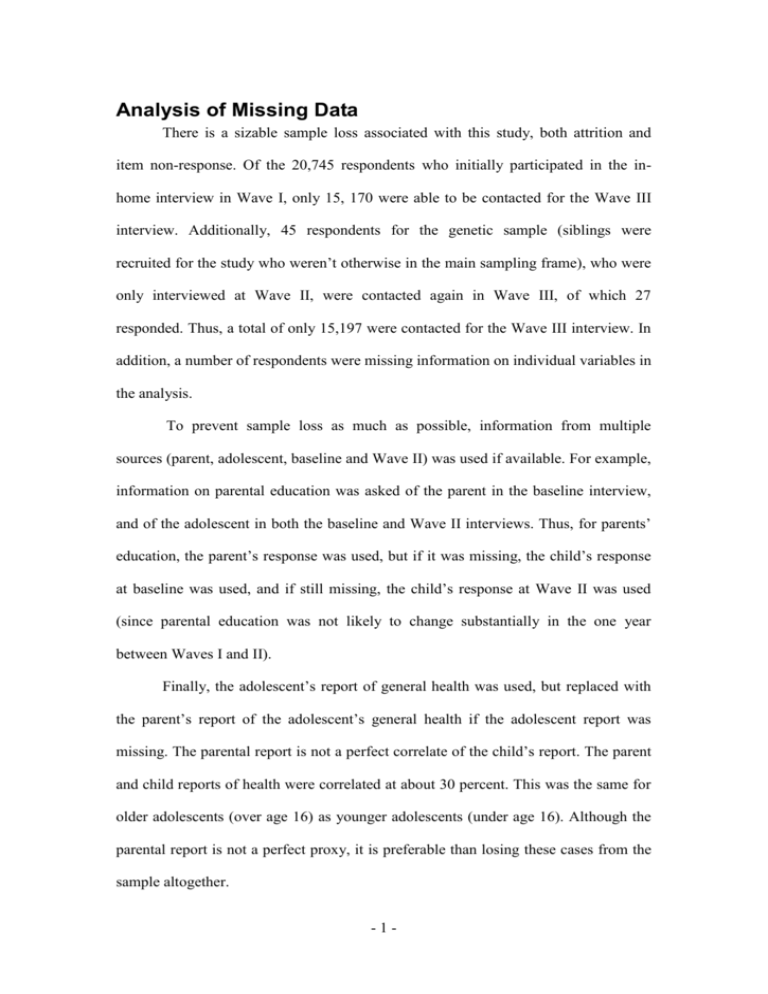
Analysis of Missing Data
There is a sizable sample loss associated with this study, both attrition and
item non-response. Of the 20,745 respondents who initially participated in the inhome interview in Wave I, only 15, 170 were able to be contacted for the Wave III
interview. Additionally, 45 respondents for the genetic sample (siblings were
recruited for the study who weren’t otherwise in the main sampling frame), who were
only interviewed at Wave II, were contacted again in Wave III, of which 27
responded. Thus, a total of only 15,197 were contacted for the Wave III interview. In
addition, a number of respondents were missing information on individual variables in
the analysis.
To prevent sample loss as much as possible, information from multiple
sources (parent, adolescent, baseline and Wave II) was used if available. For example,
information on parental education was asked of the parent in the baseline interview,
and of the adolescent in both the baseline and Wave II interviews. Thus, for parents’
education, the parent’s response was used, but if it was missing, the child’s response
at baseline was used, and if still missing, the child’s response at Wave II was used
(since parental education was not likely to change substantially in the one year
between Waves I and II).
Finally, the adolescent’s report of general health was used, but replaced with
the parent’s report of the adolescent’s general health if the adolescent report was
missing. The parental report is not a perfect correlate of the child’s report. The parent
and child reports of health were correlated at about 30 percent. This was the same for
older adolescents (over age 16) as younger adolescents (under age 16). Although the
parental report is not a perfect proxy, it is preferable than losing these cases from the
sample altogether.
-1-
With these steps taken, however, there was still a fair bit of sample loss,
particularly among the income and parent mental health variables, which were only
asked of the parents. The final sample size was 9,872 if listwise deletion methods are
used. In addressing this problem, the first step was to determine whether it was
necessary to correct for both attrition and non-response or just non-response.
AddHealth developed sample weights to correct for attrition up to Wave III. An initial
examination showed that adolescent SES and mental health were not significantly
associated with probability of inclusion in the sample once AddHealth’s weights are
included.
Reweighting
The data were then re-weighted, to determine if bias was present due to item
non-response. This was done by designing inverse probability weights (IPW) that
account for the probability of selection into the sample [37]. The variables in the full
model predicted inclusion in the sample (p-value on significance of the full model is
<0.0001). Thus, these models were used to generate the predicted probabilities for
sample selection, which were used to generate the new weights. A logit model was
run, and the predicted probability of inclusion in the sample was calculated. The
weights were calculated as the inverse of the predicted probabilities (A/P) where A=
AddHealth’s weight, in order to account for AddHealth’s attrition correction, since it
was determined earlier that AddHealth’s sampling weights effectively account for
attrition. Both Pearson’s and Spearman’s correlations showed that the new weights
correlated very strongly to AddHealth’s original weights: the Pearson’s correlation
was 0.9861 and the Spearman’s correlation was 0.9940. Thus, any further correction
for differential due to MH and SES, beyond that implicit in AddHealth’s own
-2-
correction for differential sampling and sample loss, should lead to a modest change
in the results.
But to verify that conjecture, the models were run using the new weights, in
order to compare the results under AddHealth’s original weighting to the new weights
(Appendix Table 1, first column). The results were qualitatively similar under both
the original weighting scheme and under the re-weights. Because the re-weighted
results are similar to those under AddHealth’s, the main analyses in the paper were
reported using AddHealth’s weights, because this makes it easier to replicate this
work by other researchers.
Imputation
The above findings indicate that there is not likely to be a substantial bias
problem due to failing to correct explicitly for the sample loss as long as the sample
loss is missing at random (which, as established above, can be shown when
appropriate sample weights are used). However, there is still a loss of precision,
which can make it more difficult to obtain a statistically significant a set of results and
may make it difficult to detect subgroup differences. To address this, missing values
from parental responses were imputed. Household income and parental alcoholism,
both reported by parents, had the highest number of missing values. Imputation results
are reported in the second column and third columns of Appendix Table 1. Imputation
analysis was conducted two ways: a best-regression imputation, conducted using
Stata’s impute command, and multiple regression, conducted by Stata’s ICE
command.
In the best-regression imputation, household income was imputed using a
linear regression equation where parental education, occupation and age were used to
predict household income. Although the dependent variable in this equation,
-3-
household income, is skewed (with a long tail on the right hand side of the
distribution), no corrections to this (such as using the log of income) were made, since
the goal of this equation was to impute actual income, rather than log income.
Parental alcoholism was also imputed using a linear probability model, where the
adolescent’s CES-D score and substance use (number of substances used), as well as
the adolescent’s perception of the relationship to the parents, was used to predict
parental alcoholism. Imputation flags were then created, to identify whether the
imputed values were significantly associated with the outcome. If the flags are not
significant, this indicates that observations that were missing values on the given item
are not substantially influencing the outcome. Interactions were also created between
the key mental health and SES variables and the imputation flag. A significant
interaction term in this case would indicate that the relationship between the mental
health and/or SES variables and the outcome is different for observations with
missing information on income and parental mental health than for those not missing
this information.
The second column of Appendix Table 1 shows the results with household
income and parental mental health imputed. The non-imputed results are also
presented for comparison in the fourth column. Overall, the results are similar to the
non-imputed results. The imputation flags for household income and parental
alcoholism are not statistically significant, indicating that the imputation is not
correlated with the outcome.
Finally, a multiple imputation analysis was conducted (using Stata’s ICE
command). Household income, parental education, and parent alcoholism were
imputed using these variables along with the parent’s age and occupation and the
adolescent’s CES-D score, AOD use and whether they report feeling close to their
-4-
parents. This generated a sample size of 13,418. Imputation results are reported in the
third column of Appendix Table 1. Results are similar to the best-regression
imputation. As imputed results do not differ substantially from the original sample,
the non-imputed AddHealth sample was used in the main analyses to allow for greater
replication.
-5-
Appendix Table 1. Logistic Regression Results under Reweighting, Imputation,
and Original Results Predicting Alcohol Use in Wave III
Reweighting
(n=9872)
Parent
Alcoholism
Household
Income
(in
thousands)
Income Impute
Flag
Parent Alcohol
Impute Flag
1.046
(0.838-1.304)
1.003
(1.001-1.004)***
---
Best-regression
Imputation
(n=13,328)
1.006
(0.819-1.235)
1.003
(1.002-1.098)***
Multiple
Imputation
(n=13,418)
0.999
(0.802-1.242)
1.002
(1.001-1.004)**
Original Results
(n=9456)
0.789
(0.567-1.098)
1.110
(0.731-1.687)
--
1.015
(0.818-1.259)
1.003
(1.0011.004)***
--
--
--
Note: Dependent variables assessed at Wave III. Independent variables assessed at
Wave I. All models control for binge drinking, marijuana use, cocaine use, inhalant
use and other drug use at baseline, other mental health at baseline (CESD,
delinquency, suicidality PPVT score, gender, age, age squared, race/ethnicity, general
health, family structure (two biological parents, single parent, stepfamily,
foster/other), parent alcoholism and whether adolescent is firstborn in family. Best
regression imputation model also includes interactions between imputation flags for
income and parental alcoholism and adolescent’s mental health and substance use at
baseline.
* p<0.10, ** p<0.05, *** p<0.01
-6-