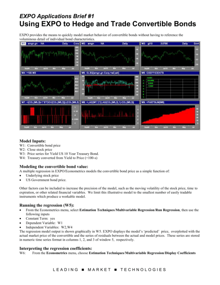
EXPO Applications Brief #1
Using EXPO to Hedge and Trade Convertible Bonds
EXPO provides the means to quickly model market behavior of convertible bonds without having to reference the
voluminous detail of individual bond characteristics.
Model Inputs:
W1:
W2:
W3:
W4:
Convertible bond price
Close stock price
Price series for Yield US 10 Year Treasury Bond.
Treasury converted from Yield to Price (=100-s)
Modeling the convertible bond value:
A multiple regression in EXPO/Econometrics models the convertible bond price as a simple function of:
 Underlying stock price
 US Government bond price.
Other factors can be included to increase the precision of the model, such as the moving volatility of the stock price, time to
expiration, or other related financial variables. We limit this illustrative model to the smallest number of easily tradable
instruments which produce a workable model.
Running the regression (W5):

From the Econometrics menu, select Estimation Techniques/Multivariable Regression/Run Regression, then use the
following inputs
 Constant Term: yes
 Dependent Variable: W1
 Independent Variables: W2,W4
The regression model output is shown graphically in W5. EXPO displays the model’s ‘predicted’ price, overplotted with the
actual market price of the convertible and the series of residuals between the actual and model prices. These series are stored
in numeric time series format in columns 1, 2, and 3 of window 5, respectively.
Interpreting the regression coefficients:
W6:
From the Econometrics menu, choose Estimation Techniques/Multivariable Regression/Display Coefficients
LEADING  MARKET  TECHNOLOGIES
The coefficients on stock price and bond price capture the sensitivity of the convertible bond price to changes in the
underlying stock and changes in interest rates. These coefficients are akin to the embedded option ‘delta’ and bond ‘duration’
of a theoretical pricing model. However, they are estimated directly from observed price responses and take on magnitudes
which reflect the specific tradable instruments used in the model.
The coefficients are displayed as the second and third numbers in Window 6. A portfolio with these weights in the underlying
stock and the government bond would track the convertible bond price as illustrated in the regression output window. The
regression constant term appears as the first number in window 6. In the context of creating a securities basket to ‘replicate’
the convertible’s price movements, the constant term would correspond to the amount of cash in the basket or, if negative, the
amount of borrowing required to hold the indicated amounts of the other securities.
Hedging Applications:
As referred to above, a portfolio constructed from the regression coefficients can be used to hedge trading positions in the
convertible bond. For a portfolio of convertibles, a hedge position can be built from a regression of the portfolio value on the
government bond and the prices of the underlying stocks of some or all of the convertibles.
Trading Applications:
The regression model can also be used to forecast movements in the spread between the convertible, its underlying stock and
the government bond. In this context, the regression estimate represents a ‘theoretical’ value of the convertible bond based
on two essential pricing factors (i.e., underlying stock price, and bond duration). If the market price of the convertible
deviates significantly from this ‘theoretical’ spread relationship, a spread trade is indicated.
Window 7 generates a short or long spread trade signal based on whether the convertible’s market value is higher or lower
than the matching basket by more than one standard deviation.
W7:
=(COL(W5,3)>1*STDEV(COL(W5,3)))-(COL(W5,3)<-1*STDEV(COL(W5,3)))
Window 8 shows the results of the daily buy or sell trade signaled by the trading rule in window 7.
W8:
=LAG(W7,1)*(LAG(COL(W5,3),1)-COL(W5,3))
Window 8 shows the cumulative trading profit which would have resulted from following this trading rule over the study
period.
W9:
=PARTSUM(W8)
Note: For presentation purposes, we estimate and test the model on a single series of data. Before implementing such a
model, it is always advisable to test the model on a time interval which is different from the one used to estimate. This can be
done with the rolling or moving regression options in EXPO/Econometrics, or by simply dividing the price series into
estimation and testing sub samples.
For more information,
Contact: Leading Market Technologies at:
One Kendall Square, Building 100
Cambridge, MA 02139 USA
Tel 617-494-4747
Fax 617-494-4788
WWW.LMT-EXPO.COM
LEADING  MARKET  TECHNOLOGIES