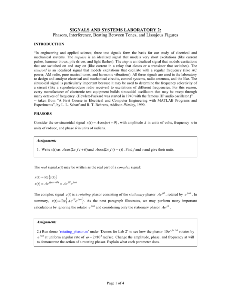
SIGNALS AND SYSTEMS LABORATORY 2:
Phasors, Interference, Beating Between Tones, and Lissajous Figures
INTRODUCTION
“In engineering and applied science, three test signals form the basis for our study of electrical and
mechanical systems. The impulse is an idealized signal that models very short excitations (like current
pulses, hammer blows, pile drives, and light flashes). The step is an idealized signal that models excitations
that are switched on and stay on (like current in a relay that closes or a transistor that switches). The
sinusoid is an idealized signal that models excitations that oscillate with a regular frequency (like AC
power, AM radio, pure musical tones, and harmonic vibrations). All three signals are used in the laboratory
to design and analyze electrical and mechanical circuits, control systems, radio antennas, and the like. The
sinusoidal signal is particularly important because it may be used to determine the frequency selectivity of
a circuit (like a superheterodyne radio receiver) to excitations of different frequencies. For this reason,
every manufacturer of electronic test equipment builds sinusoidal oscillators that may be swept through
many octaves of frequency. (Hewlett-Packard was started in 1940 with the famous HP audio oscillator.)”
-- taken from “A First Course in Electrical and Computer Engineering with MATLAB Programs and
Experiments”, by L. L. Scharf and R. T. Behrens, Addison-Wesley, 1990.
PHASORS
Consider the co-sinusoidal signal x(t )  A cos( t   ) , with amplitude A in units of volts, frequency  in
units of rad/sec, and phase  in units of radians.
Assignment:
1. Write x(t ) as A cos(2 f t   ) and A cos(2 f (t   )) . Find f and  and give their units.
The real signal x(t ) may be written as the real part of a complex signal:
x(t )  Rez (t )
z (t )  Ae j ( t  )  Ae j e j t
The complex signal z(t ) is a rotating phasor consisting of the stationary phasor Ae j , rotated by e j t . In


summary, x(t )  Re Ae j e j t . As the next paragraph illustrates, we may perform many important
calculations by ignoring the rotator e j t and considering only the stationary phasor Ae j .
Assignment:
2.) Run demo ‘rotating_phasor.m’ under ‘Demos for Lab 2’ to see how the phasor 10 e  j / 4 rotates by
e j t at uniform angular rate of   2 10 3 rad/sec. Change the amplitude, phase, and frequency at will
to demonstrate the action of a rotating phasor. Explain what each parameter does.
Page 1 of 4
INTERFERENCE
When two, or more, signals are received at a linear sensor or antenna, they will add. Depending on the
relative phase, or time alignment, of the signals, they may add constructively or destructively. A fading
radio transmission is a consequence of destructive interference of signals that are misaligned in time by
virtue of multi-path propagation. A large gain in a filter is a consequence of constructive interference of
signals that are aligned in time.
Lets elaborate by considering the addition, or interference, of two signals of the same amplitude and
frequency, but different phases (or delays):
x(t )  A cos( t  1 )  A cos( t   2 )
Now watch carefully as we use phasor calculus to simplify the effect of interference:

 Re ( Ae
 
x(t )  Re A e j1 e j t  Re A e j 2 e j t
j1

 Re Ae
j
 Ae
1  2
2
e
j 2
j
)e
j t
1  2
2

e

j

(1  2 )
2
e
j t

 Re Ae j 2 cos( / 2)e j t
 2 A cos( / 2) cos( t   ),
 2
In this formula,   1
is the average phase, and   1   2 is the phase difference. The interference
2
effect is this: when  = 0, then cos( / 2) = 1 and the output, x(t ) , is doubled in amplitude. For  = , then
cos( / 2) = 0 and the output is zeroed. For in-between values of the phase difference, the gain is between 0
and 2.
Assignment:
The function 2Acos( / 2) is called the interference pattern for two signals of equal amplitude and
frequency, and phase difference . Run the demo ‘interference_pattern.m’ under ‘Demos for Lab
2’ to plot the interference pattern. You should see something like this:
Sum of Two Sinusoids vs. Time
2
x(t)
1
0
-1
-2
-0.02
-0.015
-0.01
-0.005
Magnitude vs. psi
0
Time
0.005
0.01
0.015
0.02
Angle vs. psi
2
1
1.5
Angle
Magnitude
3.
1
0.5
0
-1
-5
0
Phase Angle (psi)
5
-5
0
Phase Angle (psi)
5
Explain what you see. Pay particular attention to the bottom two graphs, which are the magnitude
and phase of the complex interference pattern. For your own amusement, you might want to write
an interference program that accepts signals of different amplitudes.
Page 2 of 4
Assignment:
4.
Now generalize the previous development by considering the interference of these N signals:
x(t )  A cos( t )  A cos( t   )  A cos( t  2 )    A cos( t  ( N  1) )
Show that this may be written as
 sin( N / 2) j N 1

x(t )  Re  A
e 2 e j t 
 sin( / 2)

sin( N / 2)
N 1 

A
cos  t 

sin( / 2)
2


Rewrite the interference program ‘interference_pattern.m’ to plot your newly derived interference
pattern,
sin( N / 2) j
e
sin( / 2)
N 1

2
, vs. . Explain what you see. What can you say about lim
 0
sin( N / 2)
?
sin( / 2)
BEATING BETWEEN TONES
In the section on interference, we dealt with signals that had the same amplitude and angular frequency, but
different phases. Now, we are going to allow the angular frequencies to differ and study the phenomenon of
beating. As with the interference experiment, we are going to assume that the amplitudes of the signals are
equal. Then the sum of two signals with different frequencies is equal to y(t )  A cos(1t )  A cos( 2t ) .
Assignment:
5.
Run the demo ‘beating_tones.m’ from the class webpage, under ‘Demos for Lab 2’, to plot y ( t ) vs. t.
  2 
Experiment with various choices of 1 and  2 to control the beat frequency  1
 and the
2 

   2 
average frequency  1
.
 2 
Show that y(t )  A cos(1t )  A cos( 2t ) may be written as a cosine at average frequency
  2 
 1   2 
 :

 , multiplied by a cosine at the beat frequency  1
2 

 2 
    2  
    2  
y (t )  2 A cos 1
 t  cos 1
t
2
2  
 


Page 3 of 4
LISSAJOUS FIGURES
A Lissajous figure is a figure that is displayed on an oscilloscope in the ‘xy’ mode. We can simulate these
figures by graphing the equation z(t )  A1 cos( t   1)  jA2 cos( t   2) on the complex plane.
Assignment:
6.
Download and run the program ‘lissajous.m’ from the class web page under ‘Demos for Lab 2’.
Show that a Lissajous figure is just the sum of two rotating phasors, one of which rotates counterclockwise at angular frequency  and the other which rotates clockwise at angular frequency .
When is the Lissajous figure of the form Ae j e j t , and what kind of figure is this?
END NOTES:
The following m-files are located on the web page under ‘Lab 2’. These files are for your benefit. Please do
not turn in any of the results from these exercises or demos.
To get a better understanding of phasors, try the following extra exercises:
Damped Phasor:
‘damped_phasor.m’
For your own amusement, try the following extra demos:
Bicycle Wheel:
Spirograph:
Maypole:
Curves Of Unity:
‘bicycle_wheel.m’
‘spirograph.m’
‘maypole.m’
‘curves_of_unity.m’
Page 4 of 4