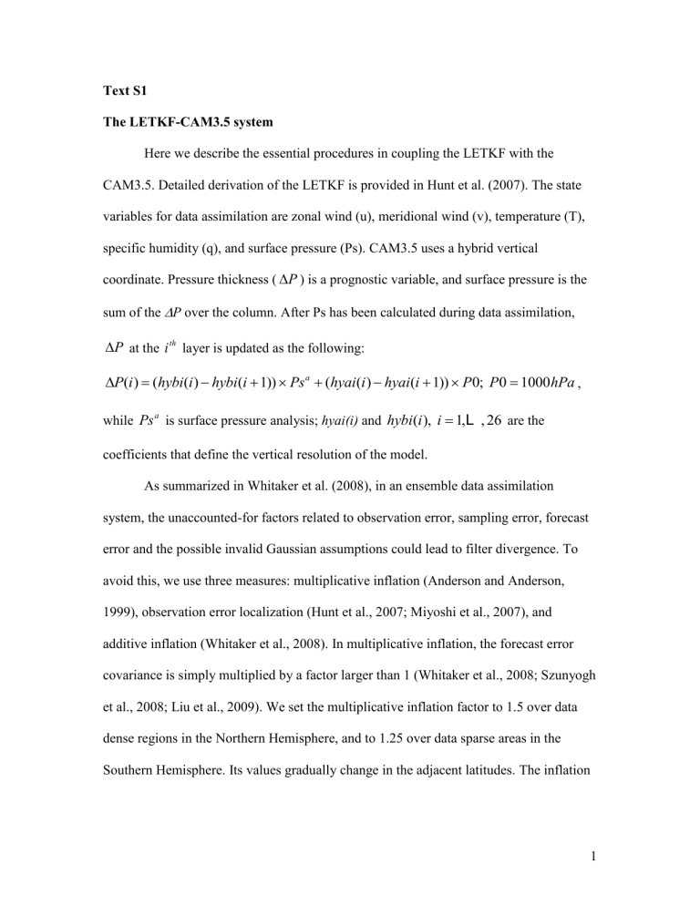
Text S1
The LETKF-CAM3.5 system
Here we describe the essential procedures in coupling the LETKF with the
CAM3.5. Detailed derivation of the LETKF is provided in Hunt et al. (2007). The state variables for data assimilation are zonal wind (u), meridional wind (v), temperature (T), specific humidity (q), and surface pressure (Ps). CAM3.5 uses a hybrid vertical coordinate. Pressure thickness (
 P
) is a prognostic variable, and surface pressure is the sum of the

P over the column. After Ps has been calculated during data assimilation,
 P
at the i th
layer is updated as the following:
 P ( i )  ( hybi ( i )  hybi ( i  1))  Ps a  ( hyai ( i )  hyai ( i  1))  P 0; P 0  1000 hPa
, while
Ps a
is surface pressure analysis; hyai(i) and hybi ( i ), i  1,
L
, 26
are the coefficients that define the vertical resolution of the model.
As summarized in Whitaker et al. (2008), in an ensemble data assimilation system, the unaccounted-for factors related to observation error, sampling error, forecast error and the possible invalid Gaussian assumptions could lead to filter divergence. To avoid this, we use three measures: multiplicative inflation (Anderson and Anderson,
1999), observation error localization (Hunt et al., 2007; Miyoshi et al., 2007), and additive inflation (Whitaker et al., 2008). In multiplicative inflation, the forecast error covariance is simply multiplied by a factor larger than 1 (Whitaker et al., 2008; Szunyogh et al., 2008; Liu et al., 2009). We set the multiplicative inflation factor to 1.5 over data dense regions in the Northern Hemisphere, and to 1.25 over data sparse areas in the
Southern Hemisphere. Its values gradually change in the adjacent latitudes. The inflation
1

factor also gradually changes over the vertical direction. It reduces to 1.25 at the top level in the NH and to 1.20 in the SH.
In the LETKF-CAM3.5 system, the selection of the observations used to update the analysis at each grid point is based on distance. Horizontally, observations within a
1500km radius around each grid point are used. Vertically, observations within 0.35 scale height are used when the grid center is below 163mb (15 th
vertical level of the model), and within 2.0 scale heights are used at the top level. The values are tapered smoothly between the 15 th
vertical level and the top level. When the distance between the observation and the grid center becomes larger than the values chosen here, the error covariance of the ensemble forecasts becomes less accurate because of the limited ensemble members. In this study, we deal with this issue by using observation error localization. We taper the inverse of observation error variance according to Blackman window function (Oppenheim and Schafer, 1989),
A ( r )  0.42
 0.5 cos
 r
L
A ( r )  0 ( r  L )
 0.08 cos
2  r
L
( r  L ) where r
is the horizontal distance between the observation and the updated grid point, and
L
is the distance where the scaling factor becomes zero. When the distance between observation and the updated analysis becomes larger, the impact of that observation on the analysis becomes smaller.
The above two measures linearly increase the magnitude of forecast/observation variance, but the enlarged variance still spans the same subspace of the original ensemble perturbations. The actual forecast error variance may span different subspace due to the unaccounted model error. To deal with the possible unaccounted subspace, we further
2

applied the third measure: additive inflation. There are different choices for the additive inflation field. For example, Whitaker et al. (2008) used scaled 6-hour analysis tendency field from NCEP/NCAR reanalysis (Kistler et al. 2001). In our case, the additive inflation fields are randomly chosen from 600 samples of analysis increments from Reanalysis-2
(Kanamitsu et al., 2002) spanning the first five months of 2003. The randomly selected inflation fields are added to the analysis ensemble before ensemble forecasts of the next assimilation cycle. The reason for this choice is that the possible systematic errors unaccounted for in the forecast error covariance have bigger impact on analysis over data dense areas, and the reduction of forecast error variance is most significant over the same areas. Since the LETKF-CAM3.5 assimilates the same observations as in Reanalysis-2, the distribution of analysis increments of Reanalysis-2 indicates the areas that the eigenspace has been most severely reduced during data assimilation and systematic errors have most significant impact in the LETKF-CAM3.5. Adding randomly sampled analysis increments to each analysis ensemble member increases the span of the perturbation subspace, especially over data dense areas.
The performance of the LETKF-CAM3.5 system
The LETKF-CAM3.5 system ( assimilation-run ) assimilates the quality-controlled raw meteorological observations assimilated in the Reanalysis-2 system (Kanamitsu et al., 2002) every 6 hours, and generates 64-member ensemble meteorological states. The assimilation period is from 01Jan 2003 till the end of 2003. Here, we only discuss results from the two time periods (i.e., from 16 January 2003 to 10 February 2003 and from 01
June 2003 to 25 June 2003) that the main text focuses on.
3

Compared to the free run , in which CAM3.5 runs freely from the same initial conditions as in the LETKF-CAM3.5 system, the Root Mean Square Error (RMSE) of the assimilation-run (solid black line in Fig S1), which assimilates meteorological observations every 6 hours, are significantly reduced for both time periods. The RMSE is calculated by verifying the results against radiosonde observations. The accuracy of zonal wind analysis from the LETKF-CAM3.5 system is between 2.5m/s and 3.5 m/s
depending on the vertical levels. The biases (dashed black line in Fig S 1) of zonal wind
are almost reduced to zero. This is also true for the other dynamical variables (not shown here).
Averaged over each time period, the spatial pattern of both geopotential height
(Fig S2) and zonal wind (Fig S3) are similar to the ECMWF interim reanalysis (Dee and
Uppala, 2009), which uses much higher resolution model and assimilates much more satellite observations than the current experiment does. The difference in geopotential height is less than 10m over most of the areas at 500hPa (Fig S4), and is less than 1m/s in zonal wind at the same level (Fig S5).
4

Fig S 1 Zonal wind RMS error (solid line) and bias (dashed line) (unit: m/s) averaged over 15 January to 10 February 2003 (left panel) and over 01 June to 25
June 2003 (right panel). Black lines are the results from the assimilation-run that assimilates meteorological observations; Grey lines are the results of the free run.
Fig S 2 Time-averaged geopotential height field (unit: m) at 500hPa from ECMWF interim reanalysis (left panels) and from the assimilation-run (right panels). Top panels are the averaged values between 15 January and 10 February 2003. Bottom panels are the averaged values between 01 June and 25 June 2003.
Fig S 3 Same as FigS2 except this is for zonal wind field (unit: m/s).
Fig S 4 The 500hPa geopotential height difference (unit:m) between the timeaveraged assimilation-run and time-averaged ECMWF interim reanalysis over two time periods: from 15 January to 10 February 2003 (top panel) and from 01 June to
25 June 2003 (bottom panel).
Fig S 5 Same s FigS4 except this is for zonal wind.
Fig S 6 64-member ensemble CO
2
forecasts (grey) and the mean of the ensemble forecasts (black) from the ensemble-run at 00June20, 2003 averaged over the tropical land (between 20

S and 20

N, top panel), and the NH land (between 20

N and 60

N, bottom panel) Blue line is from the single-run at the same time averaged over the same area.
5

Supporting references
Anderson, J. L., and S. L. Anderson, (1999), A Monte Carlo implementation of the nonlinear filtering problem to produce ensemble assimilations and forecasts. Mon.
Wea. Rev.
, 127, 2741–2758
Hunt, B., E. Kostelich, and I. Syzunogh, (2007), Efficient data assimilation for spatiotemporal chaos: A local ensemble transform Kalman filter. Physica D , 230,
112–126.
Kanamitsu M, W. Ebisuzaki, J. Woolen, S.-K.Yang, J. J. Hnilo, M. Fiorino, G. L. Potter
(2002) NCEP-DOE AMIP-II reanalysis (R-2). Bull Amer Meteorol Soc 83:1631–1643
Kistler, R., and Coauthors, (2001). The NCEP–NCAR 50-Year Reanalysis: Monthly means CD-ROM and documentation. Bull. Amer. Meteor. Soc.
, 82, 247–268.
Liu, J., H. Li, E. Kalnay, E.J. Kostelich, and I. Szunyogh, (2009) Univariate and
Multivariate Assimilation of AIRS Humidity Retrievals with the Local Ensemble
Transform Kalman Filter. Mon. Wea. Rev.
, 137 , 3918–3932.
Miyoshi, T., and S. Yamane, (2007), Local ensemble transform Kalman filtering with an
AGCM at T159/L60 resolution. Mon. Wea. Rev.
, 135, 3841–3861.
Oppenheim, A., and R. W. Schafer, (1989), Discrete-Time Signal Processing . Prentice
Hall, 879 pp.
Szunyogh, I., E. J. Kostelich, G. Gyarmati, E. Kalnay, B. R. Hunt, E. Ott, (2008),
Satterfield, E. and Yorke, J. A.: A Local Ensemble Transform Kalman filter data assimilation for the NCEP global model. Tellus A , 60 , 113-130.
Whitaker, J. S., T. M. Hamill, X. Wei, Y. Song and Z. Toth, (2008), Ensemble data assimilation with the NCEP Global Forecast System. Mon. Wea. Rev., 136, 463-482.
6