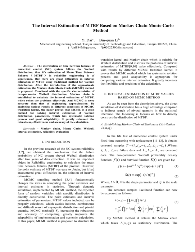
The Interval Estimation of MTBF Based on Markov Chain Monte Carlo
Method
Yi Daia ,
Bin-quan Lib
Mechanical engineering school, Tianjin university of Technology and Education, Tianjin 300222, China
b
( adai1845@qq.com,
jz05022300@sina.com)
Abstract - The distribution of time between failures of
numerical control (NC) system follows the Weibull
distribution, thus it’s estimation of Mean Time Between
Failures （ MTBF ） in reliability engineering is of
significance. But there are great difficulties in interval
estimation of MTBF using traditional method for Weibull
distribution. After the introduction of the approximate
estimation, the Markov chain Monte Carlo (MCMC) method
is proposed. Combined with the specific characteristics of
two-parameter Weibull distribution, Markov chain is
established to calculate the interval estimation of MTBF,
which solves the problems effectively. And MCMC is more
accurate than that of engineering approximation. By
analyzing various results in different conditions of MCMC
transition kernel, the paper proves that MCMC is a good
method for solving interval estimation of Weibull
distribution parameters, which has systematic solution
process and good adaptability. It greatly enhanced the
robustness, effectiveness and accuracy of the calculation.
Keywords - Markov chain, Monte Carlo, Weibull,
interval estimation, reliability evaluation
transition kernel and Markov chain which is suitable for
Weibull distribution and it solves the problems of interval
estimation of MTBF[9,10] value effectively. Compared
with results by different MCMC transition kernel, it
proves that MCMC method which has systematic solution
process and good adaptability is appropriate for
computing various interval estimates. It greatly increases
the flexibility and precision of the calculation.
II. INTERVAL ESTIMATION OF MTBF VALUES
BASED ON MCMC METHOD
As can be seen from the description above, the direct
simulation of distribution has a huge advantage compared
to indirect search of pivotal quantity in the statistical
inference. The following is focuses on how to directly
construct the distribution of MTBF.
A. Establishing Markov Chain of Stationary Distribution
L(m, )
In the life test of numerical control system under
I. INTRODUCTION
fixed time censoring with replacement [11-13], it obtains
T  (t1 , t2 ,  tr , L1 , L2 ,  Ls ) .Where,
t1 , t2 ,...tr are failure data and L1 , L2 ,  Ls are censored
censored samples
In the previous research of the NC system reliability
[1,2], we obtained the conclusions that the failure
probability of NC system obeyed Weibull distribution
after two years of data collection. It was an important
object in Reliability engineering to calculate the mean
time between failures (MTBF) of the product. However,
the point estimate of MTBF was easy to obtain, but it had
encountered great difficulties in. the solution of interval
estimation.
MCMC sampling method [3,4], fundamentally
changes the ideas in computing the point estimates and
interval estimates in statistics. Through dynamic
simulation, implemented by MCMC method, the expected
form of random variables with specific distribution is
directly constructed. The point estimates and interval
estimation of parameters, MTBF values included, can be
properly calculated, which avoids indirect, cumbersome
and difficult search of asymptotic distribution and pivotal
quantity. MCMC method[5-8], increasing the robustness
and accuracy of computing, greatly improves the
adaptability of implementation and systemic calculation,
In this paper, MCMC method is proposed to structure the
data. The two-parameter Weibull probability density
function f (t ) and Survival function S(t ) are given by:
f (t )  (mt m1 /  m ) exp[ (t /  )m ]
(1)
S (t )  exp[ (t /  ) m ]
(2)
Where, t  0 , m is the shape parameter and  is the scale
parameter.
The censored samples likelihood function can now
be expressed as follows:
r
s
i 1
j 1
L(m, )   f (ti ) S( L j )

m
r
 rm
r
t
i 1
m 1
i
(3)


t 
L 
exp    ( i ) m  exp    ( i ) m 


 i 1

 j 1

r
s
By MCMC method, it obtains the Markov chain
which takes L(m, ) as stationary distribution. The
sample obtained by Markov chain can be used for
statistical inference. For example, it obtains the samples
X (1) ,..., X (n ) through sampling from L(m, ) . If
X (1) ,..., X ( n) are the samples of Markov chain which
takes L(m, ) as stationary distribution, the Monte-Carlo
integral is still valid.
By the process above, the Markov chain which takes
L(m, ) as stationary distribution is established. Then it
obtains m and  with inverse transform. The sample
obtained by Markov chain can be used for statistical
inference.
C. Structure and implementation
Then the problem is converted into how to construct
Normal
stationary distribution of Markov chain.
Set p ( x, y )  q ( x, y ) ( x, y ) . Taking L(m, ) as
objective distribution, after choosing the proposal
distribution, q ( | x ) ,
 ( x, y ) is written as follows:
 x are initial values.
(4)
 y are proposal values, mx and
proposal
summarized as follows:
t  1,..., N :
2. Propose new values   from Unif (0.5, 0.5)
4. Calculate  ( , ) given by (6)
5. Update  (t )    with probability  ( , ) or keep the
same values with the remaining probability.
Normal
distribution
is
selected
as
proposal
distribution. The iterative step of MCMC method can be
B. Optimization of distribution parameters
summarized by the following steps:
Because the ratio  / m of Weibull distribution is
large, to ensure the iterative synchronization of two
parameters, the Jacobi's transformation [14-15] is used to
solve the two parameters first and it obtains m and 
with inverse transform.
Set u  log(  )  log( m, ) .Considering the
For
t  1,..., N :
1. Set   (m, )  ( 0(t 1) ,1(t 1) ) ,  2  (0.1, 0.1)
2. Generate   from Norm( ,  2 )
3. Calculate  ( , ) given by (6)
4. Update  (t )    with probability  ( , ) or keep the
same values with the remaining probability.
J as follows:
m
u1
 (m, )
J

 (u1 , u2 ) m
u2


  (u1 , u2 ) 


 
  (m, ) 


1

u1
Ⅲ. SIMULATION ANALYSIS

u2
u1
m
u2
m
(5)
u1

u2







1
If it establishes the Markov chain in the
37
u  space,
space. The Metropolis-Hastings
ratio  ( x, y ) is given by:
L(log (my , y ))q ( x, y ) | J ( y ) |
1
L(log 1 (mx , x ))q ( y , x ) | J ( x ) |
The censored samples of numerical control system
are obtained by the life test under fixed time censoring
with replacement. The data are given by Table Ⅰ.
TABLEⅠ
CENSORED SAMPLES (IN HOURS) OF NUMERICAL CONTROL SYSTEM
the objective distribution L(m, ) is transformed another

as
3. Calculate       
which is determined by stationary distribution L(m, ) .
distribution in
selected
distribution. The iterative step of MCMC method can be
For
So, p ( x, y ) is the transition kernel of Markov chain
Jacobian
is
1. Set   (m, )  ( 0(t 1) ,1(t 1) )
 L(my , y )q( y, x) 
min 1,

 L(mx , x )q( x, y ) 
Where, m y and
distribution
(6)
Fail
ure
Dat
a
4627
4871
848
1673
226
864
571
74
857
1758
3877
864
752
3458
3363
916
1714
1580
3769
820
2074
415
1789
813
2797
1381
606
853
4701
229
1130
93
931
2048
451
2107
356
2063
2451
999
500
4781
3329
1634
351
832
80
489
477
228
2949
65
1301
1.4
2361
1741
46
339
4429
1182
1743
36
4273
1743
2101
495
0
2354
5048
5275
2642
46
3696
3000
1545
Hollander and Proschan method[16] is selected for
goodness of fit test of the data in Table 1. It is proved that
the data obey the Weibull distribution. According to the
10000
data in Table 1, the estimation obtained by MLE 0 and
MCMC method is shown in Table Ⅱ.
2000
0
30000
3246
0.0
0.8
3143.8
Lower confidence
limit
0.89
2121.1
2074.0
1.06
2600.4
2559.6
Point estimation
Upper confidence
limit
2.0
0.8
1.25
3169.7
1.0
3190.5
1.2
1.4
1.6
1.8
m
(a)
0.8
2000
1500
1.0
3000
2500
1.2
1.4
1.6
m 4000
1.8
2000
5000
η 3500
3000
4500
0.8
1.0
50000
4500
2.0
X
1.0
0.0
0.8
2500
3500
1.0
1.2
1.4
1.6
10000
Iterations
4000
Values of MTBF
3000
2000
30000
Iterations
50000
0.8
Fig 2. The histogram and r distribution of the Weibull distribution
30000 parameters:
50000
(a) shape m , (b) scale η and (c) MTBF value
Ⅳ. CONCLUSION
10000
4500
1.8
MTBF
b
(a)
0
1.6
3.0
3500
(c)
0
1.4
3.0
8e-04
2.0
1.0
0e+00
0.0
2500
MTBF
2000
30000
Iterations
1.2
b
4e-04
X
Density
8e-04
4e-04
0e+00
3000
Values of η
1.4
1.2
1500
1500
1.0
0.8
Values of m
1.6
4000 Density
The iteration of m, η and MTBF value are shown in
Fig. 1. The histogram and distribution of m, η and MTBF
value are shown in Fig. 2.
10000
4000
η
(b) MTBF
0
4000
0.0012
3141.6
3000
η
Density
1.26
2000
X
Upper confidence
limit
1.8
0.0000
1.0
2548.8
1.6
0.0
2592.9
0.0008 0.0012
8e-04
1.0
2.0
3.0
1.06
1.4
0.0004
2073.6
1.2
4e-04
0.0
2120.0
1.0
m
3.0
0.89
Point estimation
3.0
3066
2.0
1.26
1.0
2463.0
Density
2520
0.0000
proposal
distribution
(Normal
distribution)
1.06
1.0
MCMC
method
1925.4
(c)
Fig 1. Iterations of the Weibull distribution parameters for censored
samples of numerical control system: (a) shape m and (b) scale
η.and (c) MTBF value
0.0
Proposal
distribution
(Uniform
distribution)
Lower confidence
limit
2071
50000
0e+00
Upper confidence
limit
0.89
50000
Iterations
Density
Density
Density
Point estimation
MTBF
value
Density
MLE
η
m
30000
Iterations
TABLEⅡ
RESULTS OF POINT ESTIMATION AND INTERVAL ESTIMATION
interval
estimation（90%）
Lower confidence
limit
10000
0.0012
3641
(b)
0.0008
3794
50000
Iterations
Density
744
30000
Iterations
0.0004
130
10000
0.0000
2011
10000
Iterations
0
0.0008
3.0
3551
0
50000
0.0004
2.0
1415
50000
30000
Iterations
30000
4000
25
30000
10000
3000
400
10000
4000
2915
4000
2000
0.8
1.2
Values of m
1301
0
2000
256
Values of MTBF
Censored
Data
297
Values of MTBF
1947
3000
549
Values of η
615
2000
3629
1.0
1.6
1246
Values of η
Values of m
3000
4000
0.8
1.0
1.2
1.4
1060
1.6
3042
1.0
1.2
b
1.4
1.6
1. Markov chain was established to calculate the
interval estimation of MTBF value, which solved the
difficult problem effectively. It proves that it’s more
accurate than the approximation by MLE and it ensures
the smooth implementation of reliability assessment.
2. Compared with results in the different conditions
of MCMC transition kernel, it proves that MCMC method
is appropriate for computing various interval estimates of
characteristics in reliability engineering, which has
systematic solution process and good adaptability.
MCMC method has unparalleled advantage in calculating
interval estimates and it may basically replace the
traditional methods.
3. MCMC method solves the interval estimation of
MTBF in the reliability assessment of numerical control
system effectively.
ACKNOWLEDGMENT
This work was supported by the National Natural
Science Foundation of China (50875186) and Major
projects of national science and technology
(2009ZX04014-013).
REFERENCES
[1] Dai Yi, Zhou Yunfei, Chi Xianglei, Jia Yazhou, “Failure
distribution law of a machining center and its study,”
Systems Engineering and Electronic, Vol.26, No.3, pp.413415, 2004.
[2] Zhang Haibo, Jia Yazhou, Zhou Guangwen. “Time
between failures distribution model of CNC system,”
Jourrnal of HARBIN institute of technology, Vol.37, No.2,
pp.198-200, 2005.
[3] Jim Albert. Bayesian Computation with R （ Second
Edition. New York：Springer，2009
[4] Michael S. Hamada，Alyson G. Wilson，C. Shane Reese
， Harry F. Martz. Bayesian Reliability. New York ：
Springer，2008
[5] Mao Shisong, Wang Jinglong, Pu Xiaolong, Advanced
Mathematical Statistics. China Higher Education Press,
Beijing, 1998.
[6] Andrieu, C., de Freitas, N., Doucet, A. and Jordan, M.. “An
introduction to MCMCfor machine learning.” Machine
Learning, Vol 50, pp.5-43., 2004
[7] Michael S. Hamada，Alyson G. Wilson，C. Shane Reese
， Harry F. Martz. Bayesian Reliability[M]. New York：
Springer，2008
[8] Pate-Cornell M E. “Uncertainties in risk analysis：six level
treatment. ”Reliability Engineering and System Safety，
Vol 54：pp.2-3, 1996.
[9] Erto P ， ” New practical Bayes estimates for the 2parameter Weibull distribution.” Microelectronis reliability
，Vol 34(5)：pp.789-802,1994.
[10] Athreya, K., Doss, H. and Sethuraman, J.. “On the
convergence of the Markov chainsimulation method. ”Ann.
Statist., Vol 24 pp.69– 100.,1996.
[11] Coolen F P A. On Bayesian reliability analysis with
informative priors and censoring[J]. Reliability Engineering
and System Safety， Vol 53：pp.91-98, 1996
[12] Arturo J F ， ” Bayesian inference from type II doubly
censored Raleigh data[,” statistics & Probability letters，
Vol 48：pp.393-399, 2000.
[13] Coolen F P A，Newby M J. “Bayesian reliability analysis
with imprecise prior Probabilities.” Reliability Engineering
and System Safety， Vol 43：pp.75-85, 1994.
[14] Ioannis N tzoufras. Bayesian Modeling Using WinBUGS.
Wiley，2009.
[15] Geof H. Givens, Jennifer A. Hoeting, Computational
Statistics, translation by Wang Zhaojun, Liu Minqian, Zou
Changling, Yang Jianfeng. Posts & Telecom Press, Beijing,
2009.
[16] ELISA T. LEE. Statistical Methods for Survival Data
Analysis. translation byChen Jiading, Dai Zhongwei.
Beijing：China Statistics Press，1998.