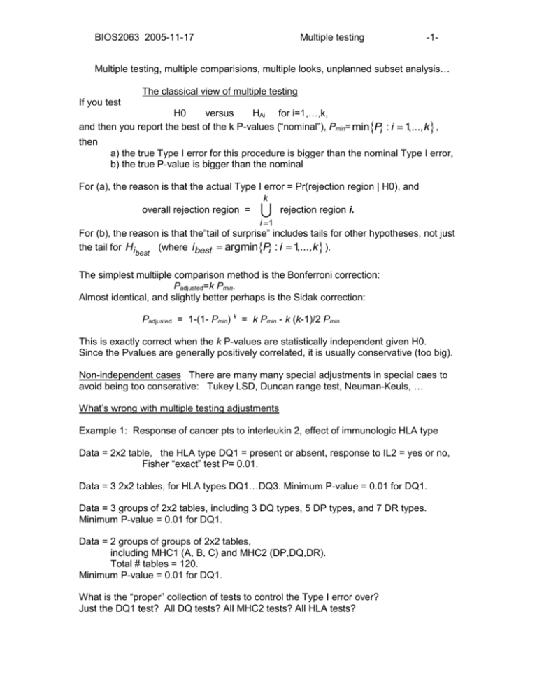
BIOS2063 2005-11-17
Multiple testing
-1-
Multiple testing, multiple comparisions, multiple looks, unplanned subset analysis…
The classical view of multiple testing
If you test
H0
versus
HAi for i=1,…,k,
and then you report the best of the k P-values (“nominal”), Pmin= minPi : i  1,..., k ,
then
a) the true Type I error for this procedure is bigger than the nominal Type I error,
b) the true P-value is bigger than the nominal
For (a), the reason is that the actual Type I error = Pr(rejection region | H0), and
k
overall rejection region =
rejection region i.
i 1
For (b), the reason is that the”tail of surprise” includes tails for other hypotheses, not just
the tail for Hi
(where ibest  argminPi : i  1,..., k ).
best
The simplest multiiple comparison method is the Bonferroni correction:
Padjusted=k Pmin.
Almost identical, and slightly better perhaps is the Sidak correction:
Padjusted = 1-(1- Pmin) k = k Pmin - k (k-1)/2 Pmin
This is exactly correct when the k P-values are statistically independent given H0.
Since the Pvalues are generally positively correlated, it is usually conservative (too big).
Non-independent cases There are many many special adjustments in special caes to
avoid being too conserative: Tukey LSD, Duncan range test, Neuman-Keuls, …
What’s wrong with multiple testing adjustments
Example 1: Response of cancer pts to interleukin 2, effect of immunologic HLA type
Data = 2x2 table, the HLA type DQ1 = present or absent, response to IL2 = yes or no,
Fisher “exact” test P= 0.01.
Data = 3 2x2 tables, for HLA types DQ1…DQ3. Minimum P-value = 0.01 for DQ1.
Data = 3 groups of 2x2 tables, including 3 DQ types, 5 DP types, and 7 DR types.
Minimum P-value = 0.01 for DQ1.
Data = 2 groups of groups of 2x2 tables,
including MHC1 (A, B, C) and MHC2 (DP,DQ,DR).
Total # tables = 120.
Minimum P-value = 0.01 for DQ1.
What is the “proper” collection of tests to control the Type I error over?
Just the DQ1 test? All DQ tests? All MHC2 tests? All HLA tests?
BIOS2063 2005-11-17
Multiple testing
-2-
Example 2: “Comparisons of a priori interest”
Testing 6 methods of measuring echocardiograms—are they equivalent?
6x5/2 = 15 comparisons
Nominal P for method B versus method C = 0.01.
But not “of a priori interest”, so P = 15 * 0.005 = 0.075, “not significant”.
But now investigator states “the comparisons of a priori interest were:
A versus D, A versus E, A versus F, D versus E, D versus F, E versus F
Now the adjusted P values for B versus C is
P = (15-6) * 0.005 = 0.045, “significant”.
Example 3: ECOG 5592 cooperative group clinical trial
Arms: (A) etoposide + cisplatin, (B) taxol+cisplatin+G-CSF, (C) taxol+cisplatin.
Should multiple comparisons adjustments be made? Which ones?
The mystery answer:
“four comparisons
B > A, C > A, B > C, C > B
so the required significance level will be
0.05 / 4 = 0.0125”.
Bayesian philosophy
Likelihood Principle 
You inference about H1 may be affected by your inference about H2,
but not by the fact that you are doing an inference about H2.
Example: Response rates dependent on hair color
Suppose that the comparisons of interest are:
H0: the response rate is 10%
vs HA: the response rate > 10%
H0D: the response rate | Dark is 10% vs HAD: the response rate | Dark > 10%
H0L: the response rate | Light is 10% vs HAL: the response rate | Light > 10%
Frequentist responses:
H0D vs HAD etc are not prespecified- don’t do them.
H0D vs HAD etc are not prespecified- do them only if H0 vs HA is significant.
Do them all, Bonferroni H0D vs HAD and H0L vs HAL by 2.
Do them all, Bonferroni H0D vs HAD and H0L vs HAL by 3.
Do them all, don’t Bonferroni, don’t tell anybody.
BIOS2063 2005-11-17
Multiple testing
-3-
A Bayesian approach:
MODEL:
logit(response | hair) =  + hair.
PRIOR:
 ~ N( 0 , ) , hair ~ N(0, ) .
Note: this is the kind of prior we needed before.
Note: corr ( dark , light )   /     .
Reasonable values might be 0 = logit(0.10),  =1,  =1.
LIKELIHOOD (approximate):
logit( pˆ )  logit( p) ~ N(0, (#responders)-1  (#nonresponders)-1)
This is a hierarchical Bayes model.
JOINT DISTRIBUTION

 logit(pdark ) 
  0 


  0 
 logit(plight ) 
~
N
  ,
 logit(pˆ

)
  0 
dark 

   
 logit(pˆ light ) 
 0












 





 
 

1
1



    nRD  nND


1
1  

 

    nRL  nNL  
POSTERIOR:
 logit(pdark ) 


 logit(plight ) 
|
  Edark
 logit(pˆdark ) 
~ N  

 Elight
ˆlight ) 
logit(
p




 ,

Vdark

 Cov
Cov
Vlight

 

The posterior means are
 Edark

 Elight
1
1


  0    
      nRD  nND



   
1
1 
    





n

n
  0   

RL
NL 
1
 logit(pˆdark )  0 


ˆ
 logit(plight )  0 
The posterior variance matrix is
Vdark

 Cov
Cov
Vlight
1
1


   
      nRD  nND

  

1
1 







    nRL  nNL 


1
 
  

   
 
For our data and the prior above,
 Edark

 Elight

 0.38 
  logit 

 0.06 

Vdark

 Cov
Cov   1.53 0.97 

Vlight   0.97 1.83 