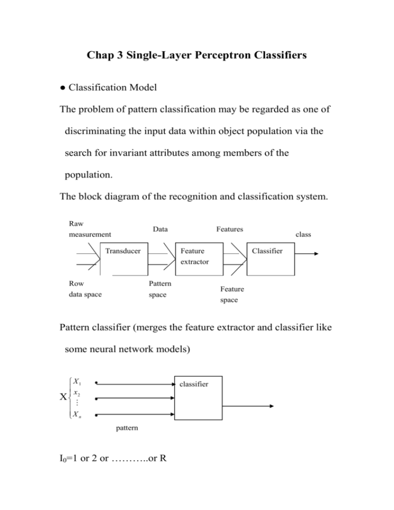
Chap 3 Single-Layer Perceptron Classifiers
● Classification Model
The problem of pattern classification may be regarded as one of
discriminating the input data within object population via the
search for invariant attributes among members of the
population.
The block diagram of the recognition and classification system.
Raw
measurement
Data
Transducer
Row
data space
Features
Feature
extractor
Pattern
space
class
Classifier
Feature
space
Pattern classifier (merges the feature extractor and classifier like
some neural network models)
 X1
x
X  2
 
 X n
classifier
pattern
I0=1 or 2 or ………..or R
Features: the compressed data from the transducer
Feature extractor: performs the reduction of dimensionality
Two simple ways of coding patterns into pattern vectors (see
Figure 3.2):
(a)
spatial object and (b) temporal object
For spatial object
io  i0 ( X ) where x  x1 , x2 , xn 
t
For temporal object
io  i0 ( X ) where x   f (t1 ), f (t2 ),, f (tn )
The pattern space is a n dimension Euclidean space En
●Decision Regions
æ1
g1(X)＞g3(X)
patterns of
class 1
X2
æ4
n=2, R=4
(-10, 10)
(20,10)
(4,6)
number of classes
Patterns
inside
decision
regions
æ1
X1
æ3
æ2
Patterns on decision surfaces
The decision function for a pattern of class j
i0(X)=j for all X  æj ,j=1,2,3,4
For space En, decision surfaces may be (n-1) dimensional
hypersurfaces.
● Discriminant Functions
During the classification step, the membership in a category
needs to be determined by the classifier based on the
comparison of R discriminant functions g1(X),
g2(X),….,gR(x),where gi(X) are scalar values.
The pattern X belongs to the i’th category, iff
gi(X)＞gj(X), for i,j =1,2,…..R, i  j
The discriminant functions gi(x) and gj(x) for contiguous
decision regions æi and æj define the decision surface between
patterns of classes i and j in En space:
gi(X)-gj(X)=0
Ex: six sample patterns, n=R=2
0,0 ,
2,0 ,
t
t
 0.5,1t ,  1,2t : class 1
1.5,1t , 1,2t : class 2
Let g(X)=-2X1+X2+2
X2
g(X)＞0
æ1
g(X)=X2-2X1+2=0
(0,0)
(2,0)
æ2
X1
1
( ,1)
2
3
( ,1)
2
(1,-2)
(-1,-2)
Decision
Surface
g(X)＜0
The classifier into R=2 classes is called the dichotomizer.
The general classification condition for the case of a
dichotomizer can now be reduced to the inspection of the sign of
the following discriminant function
g(X)=g1(X)-g2(X)
g(X)＞0 : class 1
g(X)＜0 : class 2
A single threshold logic unit (TLU) can be used to build such a
simple dichotomizer. The TLU with weights has been
introduced in Chap 2 as the discrete binary perceptron.
i0
Discriminator
1
X
i0
g(X)
pattern
g(x)
0
g
-1
Discriminant
 1

i0  sgn g ( X )  undefined

1

for g(X)  0
for g(X)  0
for g(X)  0
category
Once a general function form of the discriminant function has
been suitably chosen, discriminants can be computed using a
priori information about the classification of patterns and
their membership in classes.
● Linear Machine and Minimum Distance Classification
In general, an efficient classifier has nonlinear discriminant
functions of the inputs X1,X2,…..Xn.
ｇ1（Ｘ）
ｇ1（Ｘ）
1
ｇ2（Ｘ）
ｇ2（Ｘ） 1
2
2
Maximum
selector
X
ｇR（Ｘ）
i0
category
ｇR（Ｘ）
R
R
The use of nonlinear discriminant functions can be avoided by
changing the classifier’s feedforward architecture to the
multilayer form.
In the linear classification case, the decision surface is a
hyperplane. For example, two clusters of patterns with the
respective center points x1, x2 (vectors). The center points can
be interpreted as centers of gravity for each cluster.
We prefer that the decision hyperplane contains the midpoint
of the line segment connecting prototype points p1 and p2 and
it should be normal to the vector x1-x2.Therefore,the decision
hyperplane equation is (App. A36)

X

 t  1 

X
X2
1
2 X 
2
2

 X1
2
 0
W1 X 1  W2 X 2  |   Wn X n  Wn1  0
t 
or W X  Wn 1  0
 t 
 W  X 
    0
Wn1   1 



 W  X1  X 2

1  2
Wn1 
X 2  X1
2

2

In the case of R pairwise separable classes, there will be up to
R(R-1)/2 decision hyperplans. For R=3, there are up to three
decision hyperplanes.
Assume that a minimum-distance classification is required to
classify patterns into one of the R categories
The Euclidean distance between input pattern

x and the
prototype pattern vector Xi is


  t
 
 
x  X i  X  X i 
X  Xi
  2  
   
X  X i  X t X  2 X it X  X it X i , f o ir  1 , 2 , . R. . . . ,

independent of i
choose the smallest one
The discriminant function
  1  
g i ( X )  X i X  X it X i , for i  1,2,....., R
2
 
 g i ( X )  Wi t X  Wi ,n 1 , for i  1,2,...........R


 Wi  X i
1  
Wi ,n 1   X it X i , i  1,2,........., R
2
minimum-distance classifiers can be considered as linear
classifiers, sometimes, called linear machines.
A linear classifier
ｇ1(X)
W11
W12

1
W1,n+1
1
W21
W22
1
ｇ2(X)

W2,n+1
2
Maximum
Selector
X
WR1
ｇR(X)
WR2

R
WR,n+1
1
Ex: A linear (minimum-distance) classifier
the prototype points
i０
Response
10
2
 5
X 1   , X 2   , X 3   
2
 5
5
sol :
R3


1  
 Wi  X i , Wi,n 1   X it X i , i  1,2,3
2
 10 
 2 
 5 
W1   2 , W2    5 , W3   5 
 52
 14.5
 25
§
Nonparametric Training Concept
The sample pattern vectors X1,X2,………,Xp, called the
training seguence, are presented to machine along with the
correct response.
The classifier modifies its parameters by means of iterative,
supervised learning and its structure is usually adjusted after
each incorrect response based on the error value generated.
The adaptive linear binary classifier and its perceptron training
algorithm.
The decision surface equation in n-dimensional pattern space
is
WtX+Wn+1=0
The rewritten equation in the angmented weight space En+1 is
Wty=0
a decision hyperplane in angmented weight space.
This hyperplane always intersects the origin.
Its normal vector, which is perpendicular to the plane, is the
pattern y.
Ex: Five prototype patterns of two classes (Fig 3.11) the
normal vector will always point toward the side of the space
for which Wty＞0, called the positive side.
We look for the intersection of the positive decision regions
due to the prototypes of class 1 and of the negative decision
regions due to the prototypes of class 2.
The linear discriminant functions
g1 ( X )  10 X 1  2 X 2  52
g 2 ( X )  2 X 1  5 X 2  14.5
g 3 ( X )  5 X 1  5 X 2  25
S12 : 8 X 1  7 X 2  37.5  0
S13 : 15 X 1  3 X 2  27  0
S 23 : 7 X 1  10 X 2  10.5  0
g3 (X)＞gi(X), i=1,2
S13
g1 (X)＞gi(X) , i=2,3
P3(-5,5)
æ1
æ3
S123
P1(2,-5)
0
S23
æ2
P2(2,-5)
S12
g2 (X)＞gi(X) , i=1,3
If R linear functions of
gi(X)＞gj(X) for all

X

X
exist such that
æi, i=1,2,…….R
j=1,2,……..R, i  j
then the pattern sets æi are linearly separable.
Examples of linearly nonseparable patterns (R=2)
X2
1
-1
0
1
-1
class 1
class 2
X1