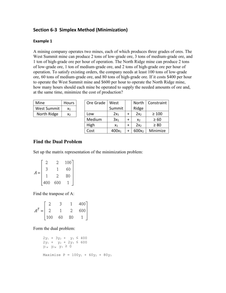
Section 6-3 Simplex Method (Minimization)
Example 1
A mining company operates two mines, each of which produces three grades of ores. The
West Summit mine can produce 2 tons of low-grade ore, 3 tons of medium-grade ore, and
1 ton of high-grade ore per hour of operation. The North Ridge mine can produce 2 tons
of low-grade ore, 1 ton of medium-grade ore, and 2 tons of high-grade ore per hour of
operation. To satisfy existing orders, the company needs at least 100 tons of low-grade
ore, 60 tons of medium-grade ore, and 80 tons of high-grade ore. If it costs $400 per hour
to operate the West Summit mine and $600 per hour to operate the North Ridge mine,
how many hours should each mine be operated to supply the needed amounts of ore and,
at the same time, minimize the cost of production?
Mine
Hours
West Summit
x1
North Ridge
x2
Ore Grade West
Summit
Low
2x1
Medium
3x1
High
x1
Cost
400x1
+
+
+
+
North Constraint
Ridge
2x2
≥ 100
x2
≥ 60
2x2
≥ 80
600x2 Minimize
Find the Dual Problem
Set up the matrix representation of the minimization problem:
Find the tranpose of A:
Form the dual problem:
2y1 + 3y2 + y3 ≤ 400
2y1 + y2 + 2y3 ≤ 600
y1, y2, y3 ≥ 0
Maximize P = 100y1 + 60y2 + 80y3
Introduce slack variables x1 and x2 into this dual problem (we'll see later why we call
them x rather than s as we have been doing):
2y1 + 3y2 +
y 3 + x1
= 400
2y1 +
y2 + 2y3
+ x2
= 600
-100y1 - 60y2 - 80y3
+ P = 0
y1, y2, y3, x1, x2 ≥ 0
Solve the Dual Problem
Solve the dual problem using the Simplex method. Find the entering variable:
Basic Variables y1 y2 y3
x1
2 3 1
x2
2 1 2
P
-100 -60 -80
x1
1
0
0
x2
0
1
0
P
0 400
0 600
1 0
x1
1
0
0
x2
0
1
0
P
Quotient
0 400 400 /2 = 200
0 600 600 / 2 = 300
1 0
Find the exiting variable:
Basic Variables y1 y2 y3
x1
2 3 1
x2
2 1 2
P
-100 -60 -80
Perform a row operation to set the pivot element to 1:
Basic Variables y1 y2 y3
x1
2 3 1
x2
2 1 2
P
-100 -60 -80
*row(1/2, [A], 1)
x1
1
0
0
x2
0
1
0
P
Operation
0 400 (1/2)*R1 → R1
0 600 (-2)*R1 + R2 →R2
1 0 100*R1 + R3 → R3
 You must set the pivot element to 1 first!
*row+(-2, Ans, 1, 2)
*row+(100, Ans, 1, 3)
The variable y1 has entered the set of basic variables:
Basic Variables
y1
x2
P
y1
1
0
0
y2 y3 x1 x2 P
3/2 1/2 1/2 0 0
200
-2 1 -1 1 0
200
90 -30 50 0 1 20,000
Select y3 as the entering variable and x2 as the exiting variable:
Basic Variables
y1
x2
P
y1
1
0
0
y2 y3 x1 x2 P
Quotient
3/2 1/2 1/2 0 0
200 200 / (1/2) = 400
-2 1 -1 1 0
200 200 / 1 = 200
90 -30 50 0 1 20,000
Since the pivot element is already one, all we have to do is perform row operations to set
remaining values in the pivot column to zero:
Basic Variables
y1
x2
P
y1
1
0
0
y2 y3 x1 x2 P
Operation
3/2 1/2 1/2 0 0
200 (-1/2)* R2 + R1 → R1
-2 1 -1 1 0
200
90 -30 50 0 1 20,000 30*R2 + R3 → R3
*row+(-.5, Ans, 2, 1)
*row+(30, Ans, 2, 3)
The variable y3 has entered the set of basic variables:
Basic Variables
y1
y3
P
y1
1
0
0
y2
5/2
-2
30
y3
0
1
0
x1 x2 P
1 -1/2 0
100
-1
1 0
200
20 30 1 26,000
Since there are no more negative values in the bottom row, we have the solution to the
dual problem. Now, the amazing thing is that we can read the solution to the original
minimization problem from the bottom row of this matrix: x1 = 20, x2 = 30, and the
minimum cost is $26,000. The mining company's standing orders can be met by running
the West Summit mine for 20 hours and running the North Ridge mine for 30 hours. This
results in the minimum operating cost of $26,000.
Graphical Interpretation
Our solution did not rely on a graphical representation of the minimization problem.
Nevertheless, it may be helpful to look at it and confirm our solution. In the graph below,
the red line represents the low-grade ore constraint (2x1 + 2x2 ≥ 100). The green line
represents the medium-grade ore constraint (3x1 + x2 ≥ 60). The blue line represents the
high-grade ore constraint (x1 + 2x2 ≥ 80).
The shaded region is the feasible region. The vertices of this region are listed in the table
below along with the number of tons of each grade of ore that is mined and the
corresponding costs of operation.
x1 Hours x2 Hours
0
5
20
80
60
45
30
0
Low-Grade Medium-Grade High-Grade
Cost
(tons)
(tons)
(tons)
120
60
120
$36,000
100
60
95
$29,000
100
90
80
$26,000
160
240
80
$32,000
Notice that the optimal solution results in just enough low-grade and high-grade ore and a
surplus of 30 tons of medium-grade ore.