CSS 590 Experimental Design in Agriculture
Lab exercise – 7th week
Orthogonal Contrasts
Regression in the ANOVA
SAS On-line Documentation
GLM Procedure
REG Procedure
Part I. Using contrast statements in a factorial experiment
An agricultural chemist suspected that the activity of root growth hormone was dependent on
temperature and concentration. He designed an experiment using two different temperature
baths of a nutrient solution containing 2 ppm, 4 ppm, and 6 ppm of the root growth hormone.
He had two assistants to help measure the root growth response so the experiment was run as
a randomized block design with two blocks.
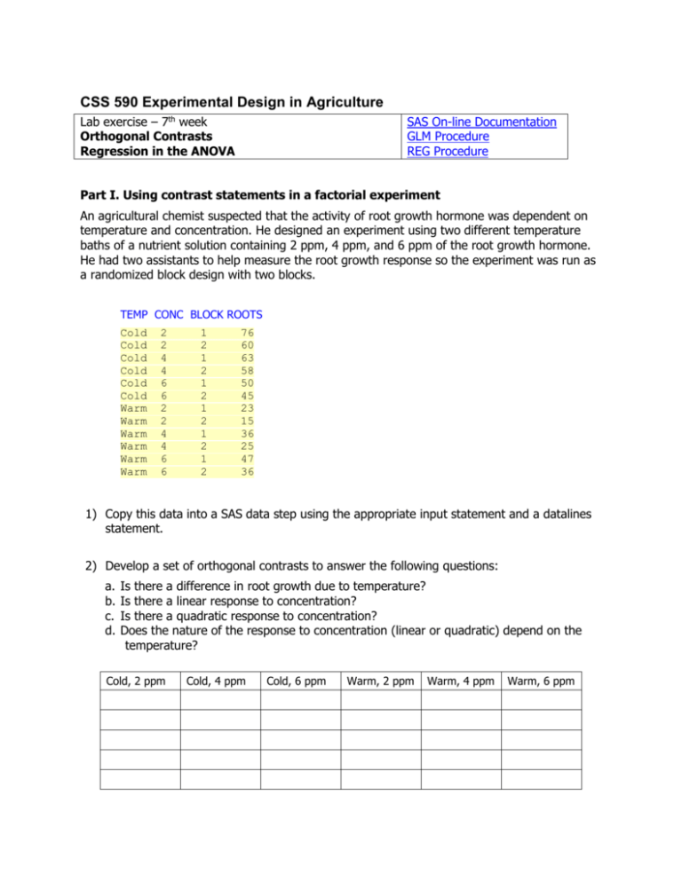
TEMP CONC BLOCK ROOTS
Cold
Cold
Cold
Cold
Cold
Cold
Warm
Warm
Warm
Warm
Warm
Warm
2
2
4
4
6
6
2
2
4
4
6
6
1
2
1
2
1
2
1
2
1
2
1
2
76
60
63
58
50
45
23
15
36
25
47
36
1) Copy this data into a SAS data step using the appropriate input statement and a datalines
statement.
2) Develop a set of orthogonal contrasts to answer the following questions:
a.
b.
c.
d.
Is there a difference in root growth due to temperature?
Is there a linear response to concentration?
Is there a quadratic response to concentration?
Does the nature of the response to concentration (linear or quadratic) depend on the
temperature?
Cold, 2 ppm
Cold, 4 ppm
Cold, 6 ppm
Warm, 2 ppm
Warm, 4 ppm
Warm, 6 ppm
3) Run a SAS program on this data to address these questions.
PROC GLM;
TITLE 'contrasts in a factorial experiment';
CLASS block temp conc;
MODEL roots = block temp conc temp*conc;
/*make sure that your coefficients correspond to the order of your
means*/
CONTRAST
CONTRAST
CONTRAST
CONTRAST
CONTRAST
'main
'conc
'conc
'temp
'temp
effect of temp' temp -1 1;
lin' conc -1 0 1;
quad' conc 1 -2 1;
x conc lin' temp*conc 1 0 -1 -1 0 1;
x conc quad' temp*conc -1 2 -1 1 -2 1;
LSMEANS conc temp;
LSMEANS temp*conc/out=new;
PROC GPLOT data=new;
TITLE 'Effect of conc and temp on root growth';
SYMBOL1 i=join v=dot;
AXIS1 label=('Root growth');
PLOT lsmean*conc=temp/ vaxis=axis1;
RUN;
4) How would you interpret the output?
5) Given these results, the chemist would like to conduct additional experiments to see if
there are differences in root growth among varieties of this plant species at cold
temperatures with 2 ppm root growth hormone. He thinks a range in root growth of about
20 g would be of practical importance. He wants to know how many replications will be
needed to detect differences of this magnitude. After running the power analysis below,
what will he conclude? How many reps would he need to detect differences at the 0.01
probability level?
PROC POWER;
Title 'determine #reps when Power=0.80, alpha=0.05';
onewayanova test=overall
groupmeans = 48|58|68
ALPHA = 0.05
stddev = 3
power = 0.80
npergroup = .
;
run;
Part II. Part I using nonclass variables
One could analyze the data from Part I by considering the quantitative factor
(concentration) to be a nonclass variable:
PROC GLM data=A;
TITLE 'regression vs contrasts in a factorial experiment';
CLASS block temp;
MODEL roots = block temp conc conc*conc temp*conc temp*conc*conc/solution;
RUN;
Part III: Regression with orthogonal polynomials compared to regression on a
quantitative variable (this section is optional!)
An experiment was conducted to determine the effect of storage temperature on seed viability.
Fifteen seed samples were obtained and three samples, selected at random from the fifteen
were stored at each of five temperatures: 10, 30, 50, 70, 90. At the end of a one year storage
period the samples were tested for germination percentage with the following results:
Temp
10
10
10
30
30
30
50
50
50
70
70
70
90
90
90
Germination
62
55
57
26
36
31
16
15
23
10
11
18
13
11
9
1) Copy this data into a SAS data step using the appropriate input statement and a datalines
statement.
2) Use Proc GLM to analyze the data as a CRD. Remember to specify that temperature is a
class variable. Are there significant differences among the Temperature treatments?
3) Use Contrast statements to determine if the effect of temperature is linear, quadratic, cubic,
or quartic (refer to the table of polynomial coefficients handed out in class).
PROC GLM;
TITLE 'Use of orthogonal polynomials';
CLASS Temp;
MODEL Germination = Temp;
CONTRAST 'Temp Linear' Temp -2 -1 0 1 2;
CONTRAST 'Temp Quadratic' Temp 2 -1 -2 -1 2;
CONTRAST 'Temp Cubic' Temp -1 2 0 -2 1;
CONTRAST 'Temp Quartic' Temp 1 -4 6 -4 1;
LSMEANS Temp / stderr out=new2;
PROC GPLOT data=new2;
PLOT lsmean*Temp;
RUN;
QUIT;
Based on your ouput, which polynomials will you retain in your model?
4) Now try running the same regression, but consider Temperature to be a continuous rather
than a class variable.
PROC GLM data=yourfile;
TITLE 'Linear Regression of germination on temperature';
MODEL Germination = Temp;
PROC GLM data=yourfile;
TITLE 'Quadratic Regression of germination on temperature';
MODEL Germination = Temp Temp*Temp;
PROC GLM data=yourfile;
TITLE 'Cubic Regression of germination on temperature';
MODEL Germination = Temp Temp*Temp Temp*Temp*Temp;
PROC GLM data=yourfile;
TITLE 'Quartic Regression of germination on temperature';
MODEL Germination = Temp Temp*Temp Temp*Temp*Temp Temp*Temp*Temp*Temp;
RUN;
Proc GLM provides direct estimates of the regression coefficients for nonclass variables.
Note how these change as we go to higher order polynomials.
Compare Type I vs Type III SS as we go to higher order polynomials. For regression
analysis using nonclass variables we generally use the Type I (sequential) SS. Type I SS
partitions the Model SS into component SS due to adding each variable sequentially to the
model in the order that they appear in the model statement. Type III SS (partial SS) determines
the SS explained be each variable after all of the other variables have been included in the
model, regardless of the order that they appear in the model statement. Compare the SS for
the quartic regression to the output from the analysis of contrasts.
What happens to MSE as we go to higher order polynomials? How does it compare to the
result from the analysis of contrasts? How do you explain the differences in the error term?
PROC REG is a general purpose regression procedure in SAS that could be used in this
example. PROC GLM or PROC MIXED are better choices if you have both class and nonclass
variables in your model. PROC REG has nine options for selecting the best model. In our
example, we could request a forward selection process to sequentially add terms to the model.
Because PROC REG cannot analyze a squared or higher order polynomial term in the model
statement, we must first create new variables representing these terms:
data four;
set three;
tempsq=temp*temp;
tempcu=temp*temp*temp;
tempqu=temp*temp*temp*temp;
PROC REG data=four;
TITLE 'Forward Selection';
MODEL Germination = Temp tempsq tempcu tempqu/SELECTION=FORWARD ss1;
RUN;
QUIT;