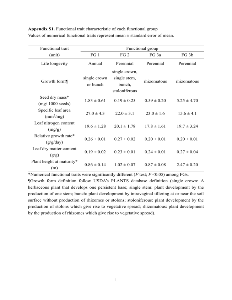
Appendix S1. Functional trait characteristic of each functional group
Values of numerical functional traits represent mean ± standard error of mean.
Functional group
Functional trait
(unit)
FG 1
FG 2
FG 3a
FG 3b
Life longevity
Annual
Perennial
Perennial
Perennial
single crown
or bunch
single crown,
single stem,
bunch,
stoloniferous
rhizomatous
rhizomatous
1.83 ± 0.61
0.19 ± 0.25
0.59 ± 0.20
5.25 ± 4.70
27.0 ± 4.3
22.0 ± 3.1
23.0 ± 1.6
15.6 ± 4.1
19.6 ± 1.28
20.1 ± 1.78
17.8 ± 1.61
19.7 ± 3.24
0.26 ± 0.01
0.27 ± 0.02
0.20 ± 0.01
0.20 ± 0.01
0.19 ± 0.02
0.23 ± 0.01
0.24 ± 0.01
0.27 ± 0.04
0.86 ± 0.14
1.02 ± 0.07
0.87 ± 0.08
2.47 ± 0.20
Growth form¶
Seed dry mass*
(mg/ 1000 seeds)
Specific leaf area
(mm2/mg)
Leaf nitrogen content
(mg/g)
Relative growth rate*
(g/g/day)
Leaf dry matter content
(g/g)
Plant height at maturity*
(m)
*Numerical functional traits were significantly different (F test; P <0.05) among FGs.
¶Growth form definition follow USDA’s PLANTS database definition (single crown: A
herbaceous plant that develops one persistent base; single stem: plant development by the
production of one stem; bunch: plant development by intravaginal tillering at or near the soil
surface without production of rhizomes or stolons; stoloniferous: plant development by the
production of stolons which give rise to vegetative spread; rhizomatous: plant development
by the production of rhizomes which give rise to vegetative spread).
1
Appendix S2. Overview of experiment (photo taken in summer 2009)
2
Appendix S3. Partitioning diversity effect
Original equation about partitioning diversity effect (Loreau & Hector 2001) was modified by
replacing response variable, yield with RCIavg (relative competitive effect on P. australis), as
follows.
Y  Yo  Ye   RYo ,i M i   RYe ,i M i  RYi M i  N RY M  N cov( RYi , M i )
i
i
i
Where,
 ∆Y = net diversity effect in term of relative competitive effect on P. australis (RCIavg)





in a mixture
Yo = observed competitive effect in the mixture
Ye = expected competitive effect in the mixture
RYo,i = Yo,i/ Mi = observed relative competitive effect of species i in the mixture
 Mi=competitive effect of species i in the monoculture
 Yo,i= Pi×Yo
 Pi = Relative cover of species i in the mixture (Note: it was originally
relative y)
RYe,i= proportion of species i in the mixture
∆RYi = RYo,I - RYe,i = deviation from expected relative competitive effect of species i
in the mixture.
In this equation, NRCM represents the complementarity effect, and N cov( RC i , Mi )
represents selection effect in terms of competitive effect.
This equation is based on the assumption that invasion resistance of each species in mixture
is proportional to “plant cover” of the species in the mixture (Co,i= Pi×Co). Because there was
significant and positive relationship between plant cover of resident species and RCIavg in
simple linear regression model (F1,55=71.96; P <0.001), the assumption was reasonable (Dr.
Michel Loreau, personal communication).
3
Appendix S4. Changes in plant cover of wetland plants and P. australis from 2009 to 2010
August
July
Legend
September
Control
1
Group 1
Group 2
2010Plant cover of Phragmites australis2009
Plant cover of Phragmites australis
Group 3
0.5
0
1
0.5
0
0
0.5
1
0
0.5
1
Plant cover of resident plants
0
0.5
Plant cover of wetland plants
Legend
 Control □ FG 1
4
 FG 2
× FG 3a
1
Appendix S5. Summary of the results of the diversity interaction models.
Diversity interaction models
(model term description)
Model 1
(species identity effect)
Model 2
(functional group identity
No. of
terms
11
3
AIC¶
Model terms (P <0.05)
model term
P
Estimate
βLolium
βBidens
-14.43 βMimulus
βScirpus
βCalamagrostis
<0.001
<0.001
0.012
0.0474
0.0475
1.190
0.712
0.396
0.308
0.311
βFG1
-16.44 βFG2
<0.001
0.012
0.971
0.339
βFG1
βFG2
-26.16
δav
<0.001
0.023
0.001
0.895
0.281
0.436
βFG1
βFG2
<0.001
0.004
<0.001
0.817
0.308
2.219
<0.001
<0.001
0.001
0.001
0.021
0.832
0.319
5.222
5.047
2.011
<0.001
0.006
<0.001
0.811
0.295
2.098
effect):
Model 3
(functional group identity
effect and average species
interaction)
Model 4
(functional group identity effect
and species interaction within
and between functional group)
Model 5
(functional group identity
effect and separate species
interactions)
4
9
-43.12
δFG1 FG3
βFG1
βFG2
δLolium
58
-41.26
Panicum
δLolium
Mimulus
δLolium Scirpus
Model 6
(functional group identity effect
and species interaction between
6
-44.46
functional group)
¶Akaike information criterion
5
βFG1
βFG2
δFG1 FG3
Appendix S6. Average similarity coefficient of wetland plants to P. australis in each
functional group. Error bar shows standard error of mean. Functional groups connected by
same letter are not significantly different from each other.
australis
Phragmitesaustralis
coefficient totoPhragmites
Similaritycoefficient
Similarity
Chart
0.9
0.8
A
A
0.7
B
0.6
0.5
C
0.4
0.3
0.2
0.1
0
FG
11
FG
22
FG
3a3a
FG
3b3b
Functional
FG group
Each error bar is constructed using 1 standard error from the
mean.
6
100.0
50
1.2
60
2.0
1.2
1.0
0.8
0.4
0.2
0.30
1.2
r= -0.36; P=0.006
0.0
0.2
0.4
0.6
RCI.avg
0.8
1.0
1.5
0.26
Relative Growth Rate (g/g/day)
0.4
1.0
0.22
1.0
1.2
Growth form
0.2
0.5
Seed mass (g/ 1000 seeds)
r= 0.51; P <0.001
0.18
0.0
0.0
0.2
0.4
0.6
RCI.avg
0.8
1.0
(h)
stoloniferous
Rhizomatous
0.0
(f)
0.0
0.0
0.2
0.4
C
single crown
r= 0.59; P <0.001
150
0.6
1.2
1.0
0.8
RCI.avg
BC
Stoloniferous
perennial
100
Plant cover (%)
AB
Bunch
(g)
0.8
1.0
40
A
Single crown
1.2
30
0.6
1.2
1.0
0.8
0.6
0.0
0.2
0.4
RCI.avg
B
(e)
Life longevity
RCI.avg
20
Plant height (cm)
A
annual
50
0.2
10
Biomass (g/pot)
(d)
0
0.0
0
0.8
20.0
0.6
5.0
RCI.avg
1.0
r= 0.79; P <0.001
0.6
RCI.avg
0.8
0.6
RCI.avg
0.2
0.0
0.2
(c)
0.4
1.2
r= 0.61; P <0.001
0.4
0.8
0.6
0.4
0.0
0.2
RCI.avg
(b)
1.0
(a) r= 0.77†; P <0.001‡
1.0
1.2
Appendix S7. Relationship between plant traits and biotic resistance (RCIavg) in the first
experiment. Performance trait (from experiment): (a) biomass, (b) plant height, and (c) plant
cover; Functional traits (from TRY trait database): (d) life longevity, (e) growth form, (f)
RGR, (g) seed mass, and (h) LDMC. Solid line represents linear regression fit (log-scale was
used in case of biomass). Means connected by same letter are not significantly different from
each other in ANOVA test (life longevity: F1,29=63.83; P<0.001; growth form: F3,27=10.81;
P<0.001). Only functional traits that have significant relationship with RCIavg are shown. †r
values represent Pearson correlation coefficient. ‡P values represent t test result on slope in
linear regression analysis.
0.20
0.25
0.30
Leaf dry matter content (g/g)
7
0.35
0.6
0.8
1.0
1.2
1.4
Plant height at maturity (m)
RCI.meanRCI.biomass RCI.shoot RCI.coverRCI.heightphrag.biomass
RCI.mean
1.0000
0.9547
0.9688
0.9368
0.8028
-0.9293
RCI.biomass
0.9547
1.0000
0.9225
0.8456
0.7005
-0.9399
RCI.shoot
0.9688
0.9225
1.0000
0.8998
0.7141
-0.8797
RCI.cover
0.9368
0.8456
0.8998
1.0000
0.6490
-0.8859
RCI.height
0.8028
0.7005
0.7141
0.6490
1.0000
-0.6618
Appendix S8. Correlations among different response variables (RCIavg, RCInumber of shoot,
phrag.biomass -0.9293
-0.9399 -0.8797 -0.8859 -0.6618
1.0000
RCIbiomass, RCIheight, RCIplant cover, and biomass of P. australis) in the experiments.
correlations
are estimated
by REML
method.
†rThe
values
represent Pearson
correlation
coefficient.
Scatterplot M atrix
1
0.5
RCIavg
RCI.mean
0
r=0.95†
-0.5
1
0.5
r=0.96
r=0.93
r=0.80 r=-0.92
r=0.92
r=0.84
r=0.70 r=-0.93
r=0.89
r=0.71 r=-0.87
r=-0.88
RCI.biomass
RCIbiomass
0
-0.5
1
0.5
RCI.shoot
RCIshoots
0
-0.5
1
0.6
RCI.cover
RCIcover
0.2
r=0.64
-0.2
1
r=-0.66
0.6
RCI.height
RCIheight
0.2
-0.2
70
50
30
10
-10
phrag.biomass
-0.5
0.5 1 -0.5
0.5 1 -0.5
0.5 1 -0.2 0.4
1 -0.2 0.4
1 -10 30 60
Multivariate year=2010 Sept
Correlations
RCI.meanRCI.biomass RCI.shoot RCI.coverRCI.heightphrag.biomass
RCI.mean
1.0000
0.9573
0.8731
0.8846
0.7843
-0.9586
RCI.biomass
0.9573
1.0000
0.7796
0.7899
0.7364
-0.9998
RCI.shoot
0.8731
0.7796
1.0000
0.7027
0.5569
-0.7819
RCI.cover
0.8846
0.7899
0.7027
1.0000
0.5923
-0.7903
RCI.height
0.7843
0.7364
0.5569
0.5923
1.0000
-0.7400
phrag.biomass -0.9586
-0.9998 -0.7819 -0.7903 -0.7400
1.0000
The correlations are estimated by REML method.
Scatterplot M atrix
0.5
0.2
-0.1
RCI.mean
8
Appendix S9. Analysing biomass of P. australis in monoculture experiments
In 2009 for the first experiment, biomass of P. australis was significantly different among
three FGs (F2,20= 25.21 , P<0.001), but it was not significantly different within each FG
(F8,20= 2.00, P=0.098). In 2010 for the first experiment, biomass of P. australis was
significantly different among three FGs (F2,20= 28.14 , P<0.001), but it was not significantly
different within each FG (F8,20= 0.96, P=0.492). In 2011 for the second experiment, biomass
of P. australis was significantly different among four FGs (F3,48= 8.96, P<0.001), but it was
not significantly different within each FG (F21,48= 1.73, P=0.059).
9
150
100
Selection effect
Net diversity effect
Complementarity effect
experiment
Net effect
mixture
Mixture
50
60
40
20
mono
Monoculture
(b)
0
Diveristy
effecteffect
(biomass
of resident
species)
(Biomass)
in mixture
Diversity
100 120
P <0.001†
80
(a)
0
Biomass
(g/pot)
plants (g/pot)
wetland species
Biomassofofresident
Appendix S10. Partitioning diversity effect based on biomass of resident species in mixture
experiment. †Contrast test result
Selection effect
Partitioning diversity effect
10