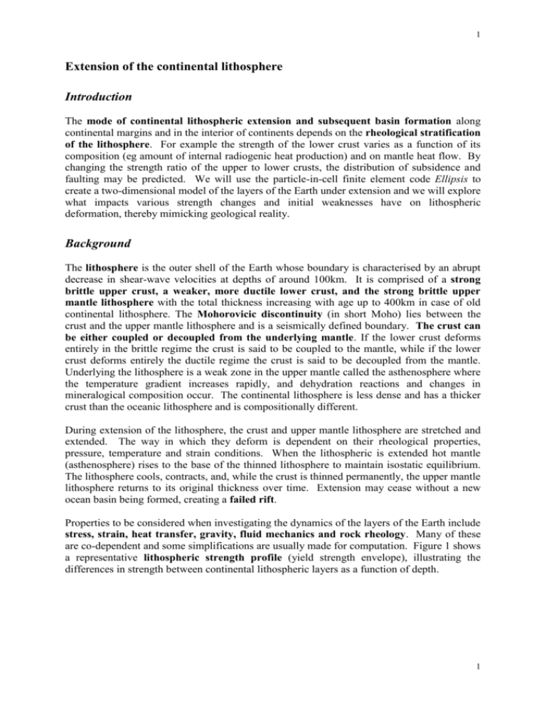
1
Extension of the continental lithosphere
Introduction
The mode of continental lithospheric extension and subsequent basin formation along
continental margins and in the interior of continents depends on the rheological stratification
of the lithosphere. For example the strength of the lower crust varies as a function of its
composition (eg amount of internal radiogenic heat production) and on mantle heat flow. By
changing the strength ratio of the upper to lower crusts, the distribution of subsidence and
faulting may be predicted. We will use the particle-in-cell finite element code Ellipsis to
create a two-dimensional model of the layers of the Earth under extension and we will explore
what impacts various strength changes and initial weaknesses have on lithospheric
deformation, thereby mimicking geological reality.
Background
The lithosphere is the outer shell of the Earth whose boundary is characterised by an abrupt
decrease in shear-wave velocities at depths of around 100km. It is comprised of a strong
brittle upper crust, a weaker, more ductile lower crust, and the strong brittle upper
mantle lithosphere with the total thickness increasing with age up to 400km in case of old
continental lithosphere. The Mohorovicic discontinuity (in short Moho) lies between the
crust and the upper mantle lithosphere and is a seismically defined boundary. The crust can
be either coupled or decoupled from the underlying mantle. If the lower crust deforms
entirely in the brittle regime the crust is said to be coupled to the mantle, while if the lower
crust deforms entirely the ductile regime the crust is said to be decoupled from the mantle.
Underlying the lithosphere is a weak zone in the upper mantle called the asthenosphere where
the temperature gradient increases rapidly, and dehydration reactions and changes in
mineralogical composition occur. The continental lithosphere is less dense and has a thicker
crust than the oceanic lithosphere and is compositionally different.
During extension of the lithosphere, the crust and upper mantle lithosphere are stretched and
extended. The way in which they deform is dependent on their rheological properties,
pressure, temperature and strain conditions. When the lithospheric is extended hot mantle
(asthenosphere) rises to the base of the thinned lithosphere to maintain isostatic equilibrium.
The lithosphere cools, contracts, and, while the crust is thinned permanently, the upper mantle
lithosphere returns to its original thickness over time. Extension may cease without a new
ocean basin being formed, creating a failed rift.
Properties to be considered when investigating the dynamics of the layers of the Earth include
stress, strain, heat transfer, gravity, fluid mechanics and rock rheology. Many of these
are co-dependent and some simplifications are usually made for computation. Figure 1 shows
a representative lithospheric strength profile (yield strength envelope), illustrating the
differences in strength between continental lithospheric layers as a function of depth.
1
2
Figure 1. Yield strength envelope for the continental lithosphere
Stress
Stress  is the internal resistance of a material to the distorting effects of an external
force with units of force per unit area. Strain  is the dimensionless ratio of change in
length to original length and describes the compressibility of a solid. In a fluid, the rate of
Ý(velocity gradient) is related to the applied stress  and the viscosity  (constant for a
strain 
given material) by the following

Ý
  
(1)
At laboratory temperatures and pressures, crustal rocks are brittle and behave elastically until
failing by fracture. An idealised elastic-perfectly plastic rheology is the model used to

approximate the behaviour of ductile materials. Elastic deformation is linear until a yield
stress is reached and maintained whereon the material deforms plastically. Just below the
Moho in figure 1 (35km), the straight edge of the yield envelope means the upper mantle
(below 35 km) deforms in a brittle fashion. However, this is also strain-rate dependent, and in
reality brittle deformation in the upper mantle only occurs when the strain rates are relatively
high, ie when the material is deformed relatively rapidly.
When temperatures reach a significant fraction of the melt temperature, atoms and
dislocations in the crystal lattice become mobile enough resulting in creep. Dislocations are
imperfections in the crystalline lattice structure and creep defines fluid behaviour over long
time scales. Even with a high viscosity, the crust is considered to behave like a fluid that
flows over geological time scales.
Newtonian flow assumes a simple linear relationship between stress and strain, the constant
of proportionality being viscosity. As soon as the viscosity is no longer constant, for example
temperature dependent, the flow is no longer strictly Newtonian. In particular, the viscosity is
modified during yielding, which makes it a function of stress, which breaks the linear
relationship, making it non-Newtonian. This behaviour can be approximated by a so-called
power-law rheology (see strain weakening), or it can be modelled more realistically by
2
3
allowing inter-dependence of variables, as is done in Ellipsis. The rheological laws used in
Ellipsis include very complicated strain and strain-rate dependencies, making the constitutive
laws very non-linear, and effectively non-Newtonian.
One of the most important parameters is the strength ratio of the upper and lower crust, at
least in the absence of pre-existing weaknesses. Extension models are also sensitive to
changes in the ratio of the relative thicknesses of the upper and lower crust. In general,
the brittle upper crust is the focus for much of the stress, which is localised in zones with
large strength ratios. Small strength ratios cause more densely spaced and widely distributed
faulting.
To approximate the brittle behaviour in the strong upper crust overlying the weak ductile
lower crust, a yield law, with a maximum shear stress  yield, describes the stress profile of
figure 1:
(2)
Ý
 yield  c 0  c p pf 
where c0 is the cohesion (yield stress at zero pressure), and cp is the pressure dependence of
Ýthe strain rate. The relative strength of the upper and
the yield stress, p is the pressure and 
lower crust can be calculated
by
integration
of equation (2), which is the area between 0 and

the maximum shear strength in figure 1.

Two different temperature dependent viscosity models can be used in Ellipsis: The complex
Arrhenius viscosity model and the simpler Frank-Kamenetskii approximation to the
Arrhenius viscosity. The Arrhenius viscosity (arr) is defined as,
1
1
 arr
 E n 
 1 n
    Exp a   
 A
 R T 
1 n
n
(3)
where A is a scaling factor, n is the stress exponent, Ea is the activation energy, R is the
universal gas constant (8.314 J/mol.K), T is the temperature (K) and ε is the strain rate.
Here however, we will only use the Frank-Kamenetskii viscosity model, which is expressed
as follows:
 T   0e T T
(4)
1
where  is the viscosity, T is the temperature (K) and 0 and T1 are constants.
By finding two values for viscosity (a and b) calculated at two different temperatures (Ta
and Tb) using the Arrhenius viscosity model you can solve the following equations to find the
constants 0 and T1 in the Frank-Kamenetskii viscosity approximation,
a (Ta )  0e T T
(5a)
b (Tb )   0e
(5b)
1 a
T1Tb
3
4
Strain Weakening
When a material is placed under high amounts of strain it can become weaker; this process is
termed strain weakening. Strain weakening is implemented in Ellipsis using the power-law
function:
f   
1  (1  a)( 
a
0)
n
  0
  0
(4)
where  is the accumulated plastic strain, 0 is the saturation strain beyond which no further
weakening takes place, n is an exponent which controls the shape of the function and a is a
maximum value of strain weakening beyond which no further weakening occurs. Figure 3
shows strain weakening behaviour for various exponents (n).
Fig 2. Strain weakening behaviour showing strength weakening from 100% to 20% after an accumulated strain
of 0.5, after which no further weakening occurs. Dashed lines show the effect of the exponential parameter (En)
on the curve (see Equation 4).
Ellipsis Background and Download Information
Ellipsis is a modelling program that simulates large deformations of materials using a finite
element method where the problem domain is represented using an Eulerian mesh, in which
Lagrangian integration points are embedded. Ellipsis has been applied to study a number of
problems, including two and three-dimensional lithospheric extension, mantle convection
modelling with a visco-elastic/brittle lithosphere, folding in finely layered visco-elastic rock
structures, and the investigation of continental geotherms, heat flow and the survival of
cratonic lithosphere through geological time.
4
5
Ellipsis is a freely available open source program, which can be downloaded from the
GeoFramework site at the California Institute of Technology (www.geoframework.org).
Ellipsis has a long history of development, mainly driven by geodynamic modeller Louis
Moresi, including not only Caltech, but also CSIRO and Monash University. Therefore,
additional web pages with Ellipsis background information and examples can be found at:
http://www.mcc.monash.edu/twiki/view/Codes/EllipsisCode
http://www.earthbyte.org/Resources/resources_ellipsis.html
Ellipsis runs on all unix-based computer operating systems (e.g. Linux, Mac OSX, Sun
Solaris, Windows (using cygwin), etc).
The Ellipsis Input File
The Ellipsis input file is a plain text file which defines all parameters we need to set up for an
Ellipsis run, ie material geometries, rheologies, boundary conditions, mesh and tracer
definitions, and output variables. The file contains an enormous number of things that the
program needs to know, but most of which don't concern us. Lines in the input file that start
with a hash mark (#) represent comments which are ignored by Ellipsis. In the following,
those sections in the input file will be highlighted that you may need to alter for your model
runs. The initial sections are:
#
#
#
#
GENERAL
ADVECTION-DIFFUSION PARAMETERS
SOLVER RELATED MATTERS
GRID POINTS
We won't have to change anything in these sections, they relate mostly to the resolution and
accuracy of the simulation. The first setup we need to look at is:
# OUTPUT FILES
The file is setup at the moment to give us four visual output files (in ppm file format – a
graphics file format like jpg, bmp and gif), ie:
PPM_files=2
The output files will display distribution of temperature, stress and strain. We also need to
extract some other data out of these models, as defined in:
# Specifications for graphical output files
We have pre-defined that we are outputting stress profiles at different points along the surface
(-more on this later).
Ellipsis Graphical User Interface
In order to make the Ellipsis program easier to use, a graphical user interface (GUI) has been
developed here at the University of Sydney. Simulations using Ellipsis must be set up by
creating a text file, called an Ellipsis input file. These files contains a long list of parameters,
5
6
in the format parameter name=parameter value. These parameter settings control all aspects
of the simulations, ranging from the types and locations of different materials in the
simulation, the rheological properties of those materials, parameters controlling how much
information Ellipsis should provide about the simulation as it executes as well as the types
and specifications of graphical output files. The parameter values can be numeric, or they can
consist of a text string. In addition, some parameters require lists of numbers or strings to be
specified.
Often groups of these parameters work together, so that it is necessary to ensure that they are
consistent with one another. For example, several parameters are used to define the materials
present at the start of the simulation, and this is done by specifying regions of various shapes.
For rectangular regions we have to define the locations of the top left and bottom right of each
region, and which material the region consists of. Because we will normally have more than
one such region in a particular simulation, we must enter lists of coordinates, so that we have
one entry for each region. It is difficult to determine the layout of the regions from such lists,
and when editing them, the user has to be careful to edit the correct number in each list. This
becomes increasingly complex as more regions, and more different region shapes are used.
Clearly it would be preferable if such lists could be replaced with a GUI that would plot the
regions graphically and allow new regions to be drawn using a mouse. Ellipsis GUI
incorporates such a system, not only for material regions, but also for boundary conditions
and tracer regions, as well as providing support for rectangular, triangular and circular
regions. The figure below illustrates the main window of the Ellipsis GUI showing the
geometrical editing capability of the GUI.
Figure 3. The visual editor pane of the GUI, showing four rectangular regions. The colour or grey-level in which
each material appears in the GUI can be specified. Here material 0 (Air) is assigned a light blue colour, material
1 (Upper crust) appears in gold, material 2 (Lower crust) appears in orange and material 3 (Mantle) appears in
red. On the left, the rectangle controls are showing, but these can be switched to show circle or triangle controls
6
7
instead. On the right are the controls for defining and choosing materials, together with a list of all the material
regions. There are also controls, which allow individual material regions to be selected and then edited, or
deleted.
To run the Ellipsis GUI, copy the following directory (using cp -r) into your home directory
from /geo/services/teaching/geos3003/Prac_extension/ellipsisgui. After you have copied it,
the GUI can be run using the command java –jar ellipsisgui.jar &. This will load the GUI and
you will see a window similar to that displayed in figure 3 above. To load an input file simply
go to File -> Load and select the input template you wish to edit.
To add a shape to the model, select the type of geometry you wish to add from the drop down
menu in the upper left of the visualisation window (rectangle, circle or triangle) and then click
and drag the mouse to add the shape. The shape that you add with be made from the currently
selected material which appears in the drop down menu to the right of the visualisation
window (Figure 3). To create a shape using a different material, simply select the material
you wish to use from the drop down menu to the right before creating the shape.
In the Visual Editor window (Figure 3) you will see a window in the bottom right called
Material Regions. This windows shows all shapes currently defined in the model. You can
manually edit the boundaries of these shapes by clicking on them and altering their
coordinates. You may also delete shapes by clicking on them in the Material Regions window
and pressing delete.
Model Resolution
Resolution of models in Ellipsis is handled using a multigrid. This technique converges on a
solution using a coarsely meshed model, and this solution is used as input for a more finely
gridded mesh, which may contain even finer meshes, and that mesh may also contain several
more nested meshes itself. This is a very computationally efficient method for solving high
resolution problems. In Ellipsis input files, different levels relate to the resolution of the finite
element mesh we are using to solve problem (Fig. 4).
Fig. 4. The meaning of levels in Ellipsis. In this example mgunitx=5 and mgunitz=3. Top: Level 0, 15
elements, middle: level 1, 60 elements, bottom: level 2, 240 elements.
Our finite element grid also contains tracers, which can move around within the mesh. They
carry information about the material properties. The more tracers we use, the higher the
resolution of the material properties we can follow through the model run.
7
8
Fig. 5. Tracer_density defined on the finest level. In this example tracer_density=4, meaning there
are four tracers/element both in the x and z direction. So in this case we have 260 elements * 16
tracers/element = 4160 tracers.
There is no hard and fast rule for how many mesh levels and tracers you should use in a given
model run. The finer the mesh and the larger the number of tracers, the longer the model run
will take. As consequence, a model run may take any time between just a few minutes to
several days (of course the geological time period covered by the run, i.e. run-length, also has
an impact on the cpu-time consumed).
The number of particles of the materials (also known as tracers), which are tracked by the
simulation can be controlled by the user. Typically the number of tracers used will be fixed
throughout the simulation area, but if necessary the number of tracers in each part of the
simulation can be varied. The maintenance of a pretty high resolution is important for your
simulations, which is why they may take a while. But, if for some reason they are taking an
extremely long time, you can set mgunitx and mgunitz to less than 8 (e.g., 5) to make things
run more quickly. Reducing ‘levels’ from 3 to 2 will greatly speed it up, but is probably too
great a sacrifice to the resolution. If the simulations are running fairly quickly, feel free to run
them for more increments (via the ‘maxstep’ parameter in the input file).
Boundary Conditions
Another factor that we have to build into the model is boundary conditions. A boundary
condition is the property of a field, either a temperate, pressure or velocity that is kept fixed
throughout the simulation, rather than being allowed to vary dynamically. These boundary
conditions can be at fixed locations, or moving, and the shape of the area to which the
boundary condition applies can vary. Commonly they are set at the edges of the simulation
area, to reflect the properties of the neighbouring spaces. We should note that stress and
velocity boundary conditions cannot both occur on the same face of the simulation
volume, if both are also in the same direction, as these are not independent factors.
However, it is possible to place orthogonal velocity and stress boundary conditions on the
same face of the simulation. By default, all velocities in a direction normal to a given face are
zero, in order to avoid a mesh that expands.
8
9
Exercise: Extension Modelling with Ellipsis
Your task
In this exercise you will:
1) Evaluate the effect of changing the coupling between the lower crust and the mantle
on the style of extension and basin formation during extension, based on Ellipsis
model run outputs I provide you with.
2) Run your own Ellipsis models (we aim for at least 4-6 runs) by focusing on two model
aspects of your choice as listed below:
a. Model with random noise
b. Model with many weak seed(s)
i. try changing the depth of the weak seed(s)
ii. try changing the strain weakening parameters
c. Model with weak fault(s)
i. try changing the angle of the fault(s)
ii. try adding multiple faults
d. Coupled model with laterally varying crustal thickness
e. Test various models with different strain rates (extension velocities)
At the same time you may vary the coupling of the crust and mantle as desired. It is
recommended that you initially only alter one set of parameters, but in your last
couple of model runs you should combine variations of parameters, eg have a couple
of preexisting faults and a thick lithospheric root somewhere in the model, or embed
material weaknesses in your model (other than faults), maybe representing a large salt
dome or a hot/weak intrusion in the upper crust together with changing the speed of
extension. Our intention is to find out how the style of deformation and basin
formation changes as a function of all these parameters (when do we get wide or
narrow, shallow or deep basins, when do we get magmatic or amagmatic, hot or cold
basins, etc etc).
3) Lastly I have provided you with a number of papers in pdf format in
/geo/services/teaching/mars3006/Prac_extension/papers.
Depending on which combinations of parameters you choose you will find various
papers where similar questions are discussed. Discuss your results based on the
papers of your choice (2-3) and make sure to include all references you have used into
a ref list in the end of your document. Convert all your movies into gif animations
(see instructions below). Refer to your gif animations in your report but leave them as
separate files.
The following example (from Artyushkov et al., Tectonophysics 320, 271-310, 2000)
illustrates the development of the Ural Mountains collision zone in the Paleozoic. The figure
shows in cross-section how many different kinds of weak and strong crustal elements were
juxtaposed during plate collision. A real world question is: what happens when such a
heterogenous crustal area is extended again some time later? What kind of basin(s) would we
expect to form?
9
10
Running Ellipsis
Copy all the files from the course directory into your home directory into your home
directory. The executable Ellipsis 2d version will be used in this practical exercise, and is
installed on the School of Geosciences Linux system. It is executed simply by typing in a
command shell:
nohup nice -10 ellipsis2d inputfile &
Where inputfile corresponds to the name of a text input file. Try it with the extension.input
file you just copied. The “nohup” command means “no hangup”. This means if you
accidentally close the command shell in which you have started this run, or even if you log
out, Ellipsis will keep on running. This is important, as runs may take several hours. The
“nice” command assigns an appropriate priority to your run, such that the computer does not
get totally bogged down from your Ellipsis run.
When you run a program using the “nohup” command, all output that would normally be
written to the screen will be written to a file called “nohup.out” in your working directory. In
order to inspect the Ellipsis screen output as it is running, type:
tail –f nohup.out
10
11
This will reproduce the screen output that Ellipsis would normally produce.
NOTE: Please only use the computer that has been assigned to you for running models.
A lot of weird stuff will scroll down the screen, but this is just normal diagnostics. Open up
another terminal and cd into the directory you left Ellipsis running in. You will eventually
notice some files being created, and they look similar to the ones you looked at in the
previous section. There are the ppm image files, also our stress profiles (out_ext.***.profiles),
and node_data (don't worry about these...). To do one simulation, it usually takes around 3hrs
depending on the machine, and its work load. Each of the following sections contains 3
simulations to do (~9hrs total, but you just let the machine work overnight etc, ie start a new
run just before you leave the prac on any given day). You will only have to cover 2 sections,
but these simulations will take a while (so make sure your input parameters are correct!!).
You can edit the inputfile with any text editor such as abiword or gedit. I recommend a simple
editor such as gedit. Make the changes, save your file (in a new directory!!! The output files
will overwrite other things of the same name). Then run Ellipsis from that directory, have a
coffee, and then check out your results. There are a number of questions for each section.
You are required to run your models in its own directory on your scratch space, as the
output takes up a lot of room. The scratch space is located in /geo/services/scratch
The following sections include a lot on the initial conditions for the model, and its boundary
conditions. The defaults are sensible to start with. For the initial extension simulation setup
we use a three-layer 2-dimensional model, including an upper crust, lower crust, and mantle
(including the mantle lithosphere and asthenosphere). These material rectangles are defined in
the Ellipsis input template under the section:
# Material distributions
The extension.input file already contains a number of pre-exsiting weakness types and
structures defined in the template. You can use this file for a template for your own ellipsis
models. The extension.input contains a single weak seed placed in the upper mantle by
default, defined as the 5th rectangle in the Material_rect=5 section. The template also
contains a fault and random diffuse weaknesses defined under the headings Fault Triangle
and Strain Triangles in the input file, however, these are commented out. If you would
like to use the weakness types defined in the model simply uncomment the relevant lines.
These weaknesses have been included in the extension.input template really as a guide for
how to implement weaknesses of this type in Ellipsis.
1.
Strength of the lower crust
Scroll down till you find the Material labelled:
#: Lower crust
The Lower Crust is Material 2. Find the viscosity parameters (Material_2_viscN0 and
Material_2_viscT1). The viscosity is a measure of strength for rocks that flow ductilely.
## coupled
Material_2_viscN0=8.985e5
Material_2_viscT1=14.4
## N0 in viscosity models
## T1 in viscosity models
11
12
## decoupled
##Material_2_viscN0=3.696e+06
##Material_2_viscT1=26
## N0 in viscosity models
## T1 in viscosity models
Note: these viscosities are non-dimensional, ie they have been scaled, along with everything
else, to input into the simulation (see appendix for how to scale real world variables such as
length in km and time in millions of years, or extension speed in km/million years.)
You can alter the coupling of the crust to the mantle by changing the viscosity parameters of
the lower crust. You can do this using the GUI or by altering the input file with a text editor.
Altering the viscosity of the lower crust so that the lower crust deforms entirely the brittle
regime couples the crust to the mantle, while altering the viscosity of the lower crust so that
the lower crust deforms entirely the ductile regime decoupled the crust from the mantle,
creating a decoupled system. To model a coupled system uncomment the “coupled” viscosity
parameters, while to model a decoupled system uncomment the “decoupled” viscosity
parameters.
Results from a simulation where the crust was coupled to the mantle and a weak seed was
placed in the upper mantle can be found here:
http://www.geosci.usyd.edu.au/users/scott/Ellipsis/Publication_Data/HuismanModels/Coupled/Single-Seed-ppm0.htm
The Ellipsis simulation templates are set up to produce two sets of image files, ending in
ppm0 and ppm1. As mentioned above, these files correspond to
ppm0 = temperature and strain localization (shaded in blue)
ppm1 = temperature only
The "ppm1" output equivalent to the model link above can be found at:
http://www.geosci.usyd.edu.au/users/scott/Ellipsis/Publication_Data/HuismanModels/Coupled/Single-Seed-ppm1.htm
and the equivalent movies can be viewed here:
http://www.geosci.usyd.edu.au/users/scott/Ellipsis/Publication_Data/HuismanModels/Coupled/movies/coupled/level5/single/coupled-hf-single-seed-huisman.00095-ppm08.7Ma-level5.gif
To look at ppm0 and ppm1 images that you produce with your model runs, type:
display filename.ppm0 &
where you need to replace filename with the actual name of your file
To see an animation of a series of figures, type:
animate out*ppm0 &
(or ppm1 depending on what you want to look at).
12
13
How does the spacing of faults vary with different strength lower crust (ie.
coupled/decoupled)? From your output images, where is the extension actually occurring
(hint: look at the blue regions in ppm0)? How does the lower crustal viscosity affect the
distribution of faulting?
We also want to look at what the stress profiles look like using MATLAB. Copy the files
profile.m and hdrload.m to the directory with your Ellipsis output. Start MATLAB by typing:
matlab &
Run the profile plotting script by typing profile into the MATLAB command prompt.
2. Distribution of faults
The examples so far have had one pre-existing weakness in the system, to act as a nucleus for
deformation. How does the distribution of faulting control the dynamics of extension? Does
the extension occur along the original faults for the entire length of the simulation? Or do the
faults just act as seed points? Does the system readjust itself if the faults cannot accommodate
the extension?
Try adding faults (using the triangle geometry) with different dips to the model. The
extension.input file already contains one fault inclined at 45˚ in the center of the model which
is commented out. This fault is defined in:
Material_trgl=1
Material_trgl_vert=3
Material_trgl_property=4
Material_trgl_x1=1.3833
Material_trgl_z1=0.3000
Material_trgl_x2=1.6167
Material_trgl_z2=0.0667
Material_trgl_x3=1.6167
Material_trgl_z3=0.0867
Here the triangle is defined by 3 vertices, which each have an x and z position. The weakness
of the fault is defined by the rheological properties of Material 4. To add more faults, use the
GUI to include more triangular weaknesses or alter the input file by hand.
NOTE: When using the GUI to add materials make sure that the new materials are aligned
with the boundaries of existing ones (eg. Do not extend a fault above the surface of the upper
crust into the air!).
3. Distributed Material weakness
Uniformly distributed random weaknesses can be included in the model in two ways. They
can be included simply by uncommenting the appropriate lines in the input file, highlighted in
red below.
## Strain Triangles - Uncomment the below lines to include random weak
seeds uniformly distributed through the crust
13
14
##Strain_trgl=40
##Strain_trgl_value=1,1,1,…
##Strain_trgl_x1=0.99,1.98,0.63,…
##Strain_trgl_z1=0.18,0.20,0.10,…
##Strain_trgl_x2=1.02,2.01,0.66,…
##Strain_trgl_z2=0.21,0.23,0.13,…
##Strain_trgl_x3=0.96,1.96,0.60,…
##Strain_trgl_z3=0.21,0.23,0.13,…
##Strain_trgl_mag=0.50,0.50,0.50,…
You can also include random weakness in your model by using the GUI to include many
random shapes of Material 4 in your model (Note: since the GUI does not yet allow you to
define regions of pre-strained material).
In model runs with random weakness seedpoints, is strain localised at all weak seedpoints, or
not? If not, how is strain distributed?
4. Intrusions/ Seeds
To include an intrusion in your model use the GUI to place a rectangular block at various
depths within the lithosphere. Using Material 4 in the GUI, simply select the rectangle shape
option and draw a small rectangle.
What happens as you change the depth of the seed in your model? How does the distribution
of faults change with an intrusion in the mantle? Does it affect the stress field? Where is strain
occuring now?
5. Thick lithospheric roots
We want to simulate the effect of a thick lower crust in one region. We do this by altering the
strength of the continental crust or by altering the temperature of regions of the model. You
can test to see what effects altering material and thermal properties have on the strength
envelope of your lithosphere by playing with the Matlab script ellispis_prac_scale.m. After
deciding which material properties you which to edit you can create a new material and add it
to your model using the GUI or by editing the text input file.
What is the effect of this thickening the crust? Now try a thinner crust in one area by adding a
small rectangle of mantle material (Material 4) at the base of the lower crust in your model.
How is having a thinner crust different from having a thicker? Is the resulting crust stronger
or weaker? How does this affect deformation?
6. Extension rates
The extension rate of the simulation is currently 4.5 x 10-10 m/s, which is equivalent to an
extension rate of 14cm/year (this is defined in the Ellipsis input template by the BCmoveX1v
variable). Try changing the velocity in the model. Using the GUI go to the Boundary
Conditions option in the Visual Editor window and click the Boundary Settings button, where
you will be able to alter the extension velocity of the right face of the model.
14
15
How does the style of deformation vary? Are the stresses greater or less? Is the
strain/deformation more or less localised? Does any layer preferentially deform more?
Gif Animations
To make a gif animation of a set of ppm output files (you will have 2 sets of ppm files for
each model run, ending with ppm0 and ppm1:
ppm2gif.mk 0
Will run a script to take all files in your working directory ending with ppm0 and turn them
into a gif animation, whereas
ppm2gif.mk 1
will do the same for all files ending with ppm1 etc.
Recommended Reading for Extension Modelling
Dyksterhuis, S., Rey, P., Müller, R.D., and Moresi, L. in press, Initial Weakness Controls on Rift
Architecture: Implications for the Iberian-Newfoundland Margin, in: MARGINS Theoretical and
Experimental Earth Science, eds: Karner, G., Manatschal, G. and Pinheiro, L., Columbia
University Press.
Harry amd Grandell, in press, A Dynamic Model of Rifting Between Galicia Bank and Flemish Cap
During Opening of the North Atlantic Ocean, in: MARGINS Theoretical and Experimental
Earth Science, eds: Karner, G., Manatschal, G. and Pinheiro, L., Columbia University Press.
Gartrell, A.P., 2000, Rheological controls of extensional styles and the structural evolution of the
Carnarvon Basin, Northwest Shelf, Australia, Australian Journal of Earth Sciences, 47, 231-244.
Lavier and Manatschal, 2006, A mechanism to thin the continental lithosphere at magma-poor
margins, Nature, 440, 324-328.
Manatschal, 2004, New models for evolution of magma-poor rifted margins based on a review of data
and concepts from West Iberia and the Alps, International Journal of Earth Sciences, 93, 432466.
Michon, L. and Merle, O., 2003, Mode of lithospheric extension: conceptual models from analogue
modelling, Tectonics, 22 (4).
Wijns et al., 2005, Mode of crustal extension determined by rheological layering, Earth and Planetary
Science Letters, 236, 120-134.
15
16
Appendix – Non-Dimensional Scaling
The Ellipsis model input parameters are scaled from real world values into dimensionless values in order to
minimise computation time and increase the accuracy of the solution. We use the non-dimensional scaling
approach given by:
E N S
Equation (1)
where E is a dimensionless Ellipsis variable, N is the dimensional real world parameter and S is a dimensional
scaling factor.
Scaling from real model length dimensions of 450km wide by 150km deep is done using a length scaling factor
(SL) of 1.5 x 105 m resulting in non-dimensional model geometry of 3 units wide by 1 unit deep.
Using a Thermal diffusivity scaling factor (S) of 1 x 10-6 a time scaling factor (St) can be found using:
St  SL S
2
Equation (2)
With a viscosity scaling factor (S) of 1 x 1021 Pa and a gravity scaling factor (Sg) of 1 m/s2, a density scaling
factor (S) can be found:
S 
S g  S L  St
S
Equation (3)
Using a velocity scale (Su) defined by:
Su  S L St
Equation (4)
a non-dimensional velocity of 67.5 is calculated to achieve a real world strain rate of 1e-15s-1 over the length of
the model.
Temperature is scaled between non-dimensional values of 0.17 and 1 corresponding to temperatures of 273K
and 1603K respectively using a temperature scale (ST) of 1603K.
For more in-depth information concerning scaling please consult the MATLAB scaling script
ellispis_prac_scale.m.
16