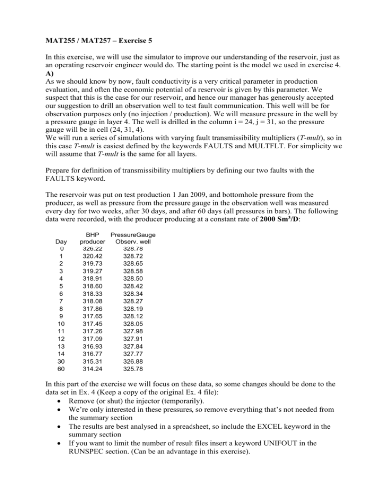
MAT255 / MAT257 – Exercise 5
In this exercise, we will use the simulator to improve our understanding of the reservoir, just as
an operating reservoir engineer would do. The starting point is the model we used in exercise 4.
A)
As we should know by now, fault conductivity is a very critical parameter in production
evaluation, and often the economic potential of a reservoir is given by this parameter. We
suspect that this is the case for our reservoir, and hence our manager has generously accepted
our suggestion to drill an observation well to test fault communication. This well will be for
observation purposes only (no injection / production). We will measure pressure in the well by
a pressure gauge in layer 4. The well is drilled in the column i = 24, j = 31, so the pressure
gauge will be in cell (24, 31, 4).
We will run a series of simulations with varying fault transmissibility multipliers (T-mult), so in
this case T-mult is easiest defined by the keywords FAULTS and MULTFLT. For simplicity we
will assume that T-mult is the same for all layers.
Prepare for definition of transmissibility multipliers by defining our two faults with the
FAULTS keyword.
The reservoir was put on test production 1 Jan 2009, and bottomhole pressure from the
producer, as well as pressure from the pressure gauge in the observation well was measured
every day for two weeks, after 30 days, and after 60 days (all pressures in bars). The following
data were recorded, with the producer producing at a constant rate of 2000 Sm3/D:
Day
0
1
2
3
4
5
6
7
8
9
10
11
12
13
14
30
60
BHP
PressureGauge
producer
Observ. well
326.22
328.78
320.42
328.72
319.73
328.65
319.27
328.58
318.91
328.50
318.60
328.42
318.33
328.34
318.08
328.27
317.86
328.19
317.65
328.12
317.45
328.05
317.26
327.98
317.09
327.91
316.93
327.84
316.77
327.77
315.31
326.88
314.24
325.78
In this part of the exercise we will focus on these data, so some changes should be done to the
data set in Ex. 4 (Keep a copy of the original Ex. 4 file):
 Remove (or shut) the injector (temporarily).
 We’re only interested in these pressures, so remove everything that’s not needed from
the summary section
 The results are best analysed in a spreadsheet, so include the EXCEL keyword in the
summary section
 If you want to limit the number of result files insert a keyword UNIFOUT in the
RUNSPEC section. (Can be an advantage in this exercise).
What is the best way to use the data above to find an estimate of T-mult? (Hint: Start with
Darcy’s law and think of physical implications of it)
If you run some simulations with “random” T-mult-values you will probably find that
irrespective of the quality of the match for the first two weeks, you can’t possibly match the last
two measurements (simulated pressure too low). Any good reason for this?
If your mind visited the concept of aquifers in this process, you’re on the right track.
The pressure trend clearly indicates that there’s more energy available than we have in our
model, and this must be because the reservoir is connected to an aquifer. We have a pretty good
idea of where and how, as the aquifer should be an extension into the water zone, but we’re
uncertain about the size of it.
Define a numerical aquifer that connects to the western edge of the reservoir. Use two grid
blocks for the aquifer, with porosity 0.28 and permeability 400 mD, and at depths 3000 and
3500 m SMSL (sub mean sea level). The aquifer cross-sectional area is 5km x 450m. The
aquifer connects to all active blocks with I=1. Total aquifer length, Aq-length, is unknown, and
shall be determined.
Insert the necessary keywords to include this aquifer in the model.
So now we have a double challenge – to determine both T-mult and aquifer size from the
pressure values above.
Intuitively, how do you assume the aquifer will influence the pressure trend? And what will the
effect of T-mult be? Can these two effects be isolated and studied separately?
To test your sense of intuition, run some simulations with systematic variation of T-mult and
Aq-length. Do your results support your intuition?
Suggest a scheme to determine (estimate) T-mult and Aq-length without needing to do too many
simulations.
You should end up with estimates which you can use in the rest of the exercise.
B)
We will then try to improve the production scheme we had at the end of Ex. 4.
To better understand the way fluids are flowing in the reservoir, we will subdivide it into fluidin-place regions, using the FIPNUM keyword.
First divide the reservoir into three areas. Area 1 will be NE of fault 1, area 3 west of fault 2,
and area 2 between the faults. Vertically, the reservoir is divided into three zones. Zone 1 is
layers 1 and 2, zone 2 is layers 3 and 4, and zone 3 is layers 5 and 6.
Define the regions by:
regions 1-3 as area 1, zones 1-3.
regions 4-6 as area 2, zones 1-3.
regions 7-9 as area 3, zones 1-3.
To increase production rates, we need more producing wells, and also some injectors to support
them. The producers will be placed along a line in the upper part of the reservoir, the injectors
in the water zone. Keep the two wells from Ex. 4, and use the same well completion and target
data (as in Ex. 4) for the rest of the wells.
Define three new producers, in blocks (i, j, k1-k2). OP2: (23,3, 1-5, OP3: (28,10, 3-6), and
OP4: (28,23, 3-6); and two new injectors WI2 (1,18,1-6) and WI3 (1,38,1-6).
The wells will be put on injection / production:
WI2 and OP2: 1. Jul. 2010
WI3 and OP3: 1. Jan. 2011
OP4:
1. Jul. 2011
Now we have more than one producer we don’t want the run to stop if a well is shut in. Change
the WECON keyword accordingly.
We do, however want the run to stop if all producers are shut. To achieve that use the GECON
keyword – group economic control. Define minimum field oil rate as 200 Sm3/day, and max
field water cut as 0.8. If these are violated the worst offending well shall be shut, and if all wells
are shut the run shall terminate.
Next we will add several new summary keywords. As we now have more wells, the field oil
rate is no longer equal to well oil rate, so all the keywords for production rates, production
totals, injection rates, injection totals, and water cut should be defined for both field and
appropriate wells. Also store flowing bottomhole pressures for all wells. Insert summary
keywords for region oil in place, region oil efficiency, and some region flux keywords, for the
nine regions. We’ll also want to compare run times and convergence for this run and coming
exercises. Insert summary keywords for recording (at least) CPU used, CPU pr time step, and
time step lengths.
At this stage run the simulation, and if everything is OK, look at the performance. You
probably got some “not fully converged” warnings. Recall that problems could be expected
when new wells were introduced. Consider inserting additional TUNING keywords at
appropriate dates.
Extend the simulation time with another couple of years, e.g. to 1.1. 2035. (Doesn’t matter if we
go “too far” since the simulation will stop at group economic limits anyway.)
Spend a little time looking at the simulation in FloViz and OFFICE / GRAF. It’s beginning to
look like a real case...
C)
Define a horizontal well WPH1 in the centre of layer 3, with wellhead at the heel, in cell
(9, 16, 3) and toe in cell (9, 34, 3). The well path is a straight line between heel and toe (in XYview), and is completed in all cells it penetrates. WPH1 is set on production 1. Jan. 2012.
Run this case.
It is recommended to model horizontal wells in combination with local grid refinement. Define
an LGR which subdivides all the blocks that WPH1 passes through into 3 x 3 x 3 LGR-blocks.
Change other keywords as necessary to define the well on the local grid.
Run this case and compare with the non-LGR case. Conclusion??