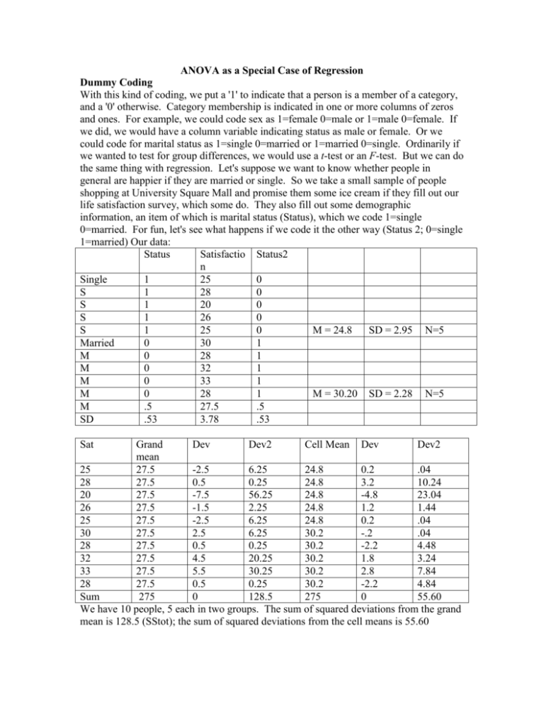
ANOVA as a Special Case of Regression
Dummy Coding
With this kind of coding, we put a '1' to indicate that a person is a member of a category,
and a '0' otherwise. Category membership is indicated in one or more columns of zeros
and ones. For example, we could code sex as 1=female 0=male or 1=male 0=female. If
we did, we would have a column variable indicating status as male or female. Or we
could code for marital status as 1=single 0=married or 1=married 0=single. Ordinarily if
we wanted to test for group differences, we would use a t-test or an F-test. But we can do
the same thing with regression. Let's suppose we want to know whether people in
general are happier if they are married or single. So we take a small sample of people
shopping at University Square Mall and promise them some ice cream if they fill out our
life satisfaction survey, which some do. They also fill out some demographic
information, an item of which is marital status (Status), which we code 1=single
0=married. For fun, let's see what happens if we code it the other way (Status 2; 0=single
1=married) Our data:
Status
Satisfactio Status2
n
Single
1
25
0
S
1
28
0
S
1
20
0
S
1
26
0
S
1
25
0
M = 24.8
SD = 2.95 N=5
Married
0
30
1
M
0
28
1
M
0
32
1
M
0
33
1
M
0
28
1
M = 30.20 SD = 2.28 N=5
M
.5
27.5
.5
SD
.53
3.78
.53
Sat
Grand
Dev
Dev2
Cell Mean Dev
Dev2
mean
25
27.5
-2.5
6.25
24.8
0.2
.04
28
27.5
0.5
0.25
24.8
3.2
10.24
20
27.5
-7.5
56.25
24.8
-4.8
23.04
26
27.5
-1.5
2.25
24.8
1.2
1.44
25
27.5
-2.5
6.25
24.8
0.2
.04
30
27.5
2.5
6.25
30.2
-.2
.04
28
27.5
0.5
0.25
30.2
-2.2
4.48
32
27.5
4.5
20.25
30.2
1.8
3.24
33
27.5
5.5
30.25
30.2
2.8
7.84
28
27.5
0.5
0.25
30.2
-2.2
4.84
Sum
275
0
128.5
275
0
55.60
We have 10 people, 5 each in two groups. The sum of squared deviations from the grand
mean is 128.5 (SStot); the sum of squared deviations from the cell means is 55.60
(SSwithin), and difference must be SSbetween = 128.5-55.60 = 72.90. To test for the
difference we find the ratio of the two mean squares:
F
MS B 72.9 / 1 72.9


 10.49
MSW 55.6 / 8 6.95
Or we could compute a t-test by
t
Y1  Y2
y y
1
1
  
n1  n2  2  n 1 n2 
2
1
t
2
2
24.8  30.2
34.8  20.8  1 1 

5  5  2  5 5 

 5.4
 3.2387
1.667
And if we square this result, we get 10.49, which is our value for F (recall that F = t2).
To compute regressions, we find that:
X
xbar
x-xbar dev*dev
Y
Ybar
y-ybar
xy
1
1
1
1
1
0
0
0
0
0
0.5
0.5
0.5
0.5
0.5
0.5
0.5
0.5
0.5
0.5
0.5
0.5
0.5
0.5
0.5
-0.5
-0.5
-0.5
-0.5
-0.5
0.25
0.25
0.25
0.25
0.25
0.25
0.25
0.25
0.25
0.25
25
28
20
26
25
30
28
32
33
28
27.5
27.5
27.5
27.5
27.5
27.5
27.5
27.5
27.5
27.5
-2.5
0.5
-7.5
-1.5
-2.5
2.5
0.5
4.5
5.5
0.5
-1.25
0.25
-3.75
-0.75
-1.25
-1.25
-0.25
-2.25
-2.75
-0.25
Formula
 xy
b
 x2
Status
-35.5/2.5 = -5.4
Status2
35.5/2.5 = 5.4
a  Y  bX
Y   a  bX
ssreg  b xy
27.5-(-5.4*.5)= 30.20
Y' =30.20-5.4X
-5.4(-35.5)=72.90
27.5-(5.4*.5) = 24.8
Y'=24.8+5.4X
5.4(35.5)=72.90
128.5-72.90=55.6
128.5-72.9=55.6
55.6/8 = 6.95
55.6/8=6.95
Sqrt(6.95/2.5) = 1.667
Sqrt(6.95/2.5) = 1.667
-5.4/1.667 =
-3.239
5.4/1.667 =
3.239
72.9/128.5=.5673
72.9/128.5=.5673
ssres   y 2  ssreg
sy2.x 
sy2.x
sb 
t
ssres
N  k 1
x
b
sb
r2 
ssreg
y
2
2
(.57/1)/(.43/8)=
(.57/1)/(.43/8)=
r2 / k
10.49
10.49
(1  r 2 ) / ( N  k  1)
Points to notice:
1. If we switch the vector (column) from zeros to ones (status to status 2), we just
change the sign of the deviations from the mean. This gives us b weights of equal
magnitude but opposite signs for the two analyses (status and status 2). The bulk of
the regression results are identical for the two methods of coding the category.
2. The regression equations are fit to data for zeros and ones -- the X variable only
takes on these two values.
3. When X = 0, our predicted value is the mean for that group (those designated with a
zero). When X = 1, our predicted value is the mean for that group. Look at the
regression equations for each. When single was coded 1 (status), the equation was
Y' = 30.2 - 5.4X. So when X is zero (married people), the predicted value is 30.2,
the mean for married people. When X=1 (single), the predicted value is 24.8, the
mean for single people. The b weight is equal to the difference in means between
the groups. When we code the other way (1=married), the equation is Y' =
24.8+5.4X. Now when X is zero (single), the predicted value is 24.8, the mean of
the single group. When X=1, the predicted value is 30.2, the mean of the married
group.
4. The regression results are the same as what we got using ANOVA formulas for F
and for t.
We can apply dummy coding to categorical variables with more than two levels. We can
keep the use of zeros and ones as well. However, we will always need as many columns
as there are degrees of freedom. With two levels, we need one column; with three levels,
we need two columns. With C levels, we need C-1 columns.
F