1
(D) Pulsed NMR: D_I
Inversion Recovery and T1 Relaxation
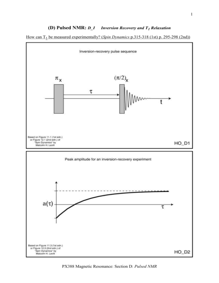
How can T1 be measured experimentally? (Spin Dynamics p.315-318 (1st) p. 295-298 (2nd))
PX388 Magnetic Resonance: Section D: Pulsed NMR
2
D_II
Spin Echoes and T2 Relaxation
What is the difference between T2 and T2*? (Spin Dynamics p.318-320 (1st) p.298-299 (2nd))
PX388 Magnetic Resonance: Section D: Pulsed NMR
3
How can T2 be measured? (Spin Dynamics p.320-325 (1st edn.) p. 299-303 (2nd edn.))
PX388 Magnetic Resonance: Section D: Pulsed NMR
4
PX388 Magnetic Resonance: Section D: Pulsed NMR
5
PX388 Magnetic Resonance: Section D: Pulsed NMR
6
D_III
Fourier Transformation and Frequency-Domain Spectra
How is the sign of the resonance offset determined? (Spin Dynamics p.81-82(1), p.73-75 (2))
PX388 Magnetic Resonance: Section D: Pulsed NMR
7
How is a time-domain NMR signal converted into a frequency-domain spectrum? (Spin
Dynamics p.101-107 (1st edn.), p.93-102 (2nd edn.))

S() =

s(t) exp(i  t) dt
0
PX388 Magnetic Resonance: Section D: Pulsed NMR
[D7]
8
D_IV
Sensitivity
What parameters determine the size of a NMR signal?
Why does adding together individual FIDs improve the signal to noise? (Spin Dynamics p.9093 (1st edn.), p.86-89 (2nd edn.))
PX388 Magnetic Resonance: Section D: Pulsed NMR
9
D_IV
Magnetic Resonance Imaging (MRI)
How can a magnetic-field gradient be used to generate a one-dimensional frequency-encoded
image? (Spin Dynamics p.325-329 (1st edn.) p. 309-312 (2nd edn.))
PX388 Magnetic Resonance: Section D: Pulsed NMR
10

Btotal = B0 + Bxgrad
= (

)k
0 =  Bz

0(x) =  (

=

[D16]
[A9]
)
[D17]
0 = 0  rf
[B2]
Set rf = 0(x = 0)

0(x) =
[D18]
PX388 Magnetic Resonance: Section D: Pulsed NMR
11
How can the imaging technique be extended beyond one dimension?
PX388 Magnetic Resonance: Section D: Pulsed NMR
12
How does phase-encoding work?
PX388 Magnetic Resonance: Section D: Pulsed NMR
13
How are frequency- and phase-encoding combined to generate a two-dimensional image?
(Spin Dynamics p.330-334 (1st edn.) p. 312-315 (2nd edn.))
PX388 Magnetic Resonance: Section D: Pulsed NMR
14
How are two-dimensional slices taken from a three-dimensional object? (Spin Dynamics
p.307-309 (2nd edn.))
PX388 Magnetic Resonance: Section D: Pulsed NMR
15
How is a gradient-echo generated? (Spin Dynamics p.306-307 (2nd edn.))
How are differences in relaxation times used to obtain image contrast?
PX388 Magnetic Resonance: Section D: Pulsed NMR
16
What is a typical imaging pulse sequence?
How can fast MRI experiments (for functional MRI, fMRI) be performed?
PX388 Magnetic Resonance: Section D: Pulsed NMR
17
(D) Pulsed NMR: Key Facts

Measurement of the longitudinal relaxation time, T1
The signal, a(), in an inversion-recovery pulse sequence: x  /2x tacq

a()  [1  2 exp(/T1)]
[D1]
For derivation of eq. [D1] see question 1 below.
The first zero crossing occurs when

zero-crossing = T1 ln{2}

[D2]
T2 and T2*
In an inhomogeneous B0 magnetic field, nuclei in different parts of the sample have different
Larmor frequencies, 0. Hence, during time periods of free precession (i.e., when no B1
magnetic field is applied), they evolve at different resonance offsets, 0.
The loss of transverse magnetisation for the nuclei in different parts of the sample is
characterised by a common transverse relaxation time, T2, according to exp{t / T2}.
However, the superposition of signals evolving at different resonance offsets, 0, causes the
total signal to be characterised by a faster apparent decay, exp{t / T2*}, corresponding to an
apparent transverse relaxation time, T2*, where T2* < T2.

Measurement of the transverse relaxation time, T2
For a spin-echo pulse sequence: /2x /2 y /2 tacq
The sandwiching of two time periods of free precession between a  pulse that inverts the
magnetisation has the consequence that evolution under a resonance offset, 0, is refocused,
i.e., the signal, a(), is independent of 0, and hence a() is the same for all nuclei in an
inhomogeneous B0 magnetic field. (For derivation, see question 2 below)
a()  exp( / T2)
PX388 Magnetic Resonance: Section D: Pulsed NMR
[D3]
18

Quadrature detection (determination of the sign of the resonance offset, 0)
Experimentally, two NMR signals that are 90 degrees out of phase with respect to each other
are obtained by mixing down the one NMR signal from the probe with two rf waveforms with
the same rf, but with relative phases, 0 and 90 (see section B).
These two NMR signals (free induction decay, FID)

FIDcos(t)  cos{0 t} exp{t / T2}
[D4]

FIDsin(t)  sin{0 t} exp{t / T2}
[D5]
constitute the real and imaginary parts of a complex time-domain signal:
s(t) = FIDcos(t) + i FIDsin(t)  [cos{0 t} + i sin{0 t}] exp{t / T2}
s(t)  exp([i 0  (1/T2)] t)

[D6]
Fourier transformation

S() =

s(t) exp(i  t) dt
[D7]
0
Fourier transformation of a complex time-domain signal  an oscillating and decaying signal
that is characterised by a precession frequency (in the rotating frame), 0, and a transverse
relaxation time, T2  gives a complex frequency-domain signal, namely an absorptive-mode
(real part) and a dispersive-mode (imaginary part) Lorentzian lineshape (see HO_D11)
centred at the frequency, 0. The full-width at half-maximum height (FWHMH) of the
absorptive-mode Lorentzian lineshape is inversely proportional to T2 (see question 4 below):
FWHMH in Hz = 1 /  T2
PX388 Magnetic Resonance: Section D: Pulsed NMR
[D10]
19

NMR signal strength
From Faraday's law, the induced voltage (i.e., the NMR signal) is proportional to the rate of
change of the magnetisation with respect to time. Using eq. [A20]
NMR Signal  N 3 B02 / T
[D12]
Importantly, NMR is quantitative, i.e., the intensity of a given resonance is proportional to the
number of spins in the sample.

Improving signal to noise
The signal-to-noise (S/N) in a NMR experiment can be improved by repeating the experiment
n times and adding the FIDs together. Since the signal is proportional to n, whereas the noise
is proportional to √n:
S/N  n
[D13]
The repetition time between experiments is determined by T1, since the thermal equilibrium
bulk magnetisation must re-establish.

Imaging and Spectroscopy
Distinction: spatial information is obtained in an imaging experiment by the use of additional
applied magnetic field gradients.
Most MRI (magnetic resonance imaging) experiments look at 1H (near 100 % natural
abundance, and the highest  of all NMR isotopes – remember that the NMR signal  3
[D12]) in water and other biofluids.

One-Dimensional Imaging
In addition to B0 (due to the strong, static superconducting magnet), a magnetic field gradient
is applied (NB: x refers to the x position, and is not a multiply sign):

Bxgrad = Gx x k
[D14]
Gx = dBz / dx
[D15]
PX388 Magnetic Resonance: Section D: Pulsed NMR
20
NB: The additional magnetic field due to a gradient coil is always in the k direction (i.e., the
same direction as B0). It is the gradient of the additional magnetic field that can be in any
direction – eq. [D15] is for an x gradient.
In a one-dimensional imaging experiment, where rf = 0(x = 0)

0(x) =  Gx x
[D18]
i.e., the precession frequency depends on the x position – this is referred to as frequency
encoding.
Therefore, the signal intensity at a given resonance offset, S(), is proportional to the density
of spins at a particular x position, i.e., the one-dimensional frequency-domain spectrum
corresponds to the projection of the spin density onto the x axis:
S()  (x)

[D19]
Two-Dimensional Imaging
A two-dimensional imaging experiment combines frequency encoding under one magnetic
field gradient (e.g., Gx) during the acquisition of the NMR signal (during a time period, t2)
with phase encoding under an orthogonal field gradient (e.g., Gy) during a time period, , of
free evolution that precedes the acquisition of the NMR signal:
S(Gx, t2) = exp{i  Gy y exp{i  Gx x t2
[D24]
A two-dimensional data set is obtained by recording a series of NMR signals for different
values of the phase-encoding magnetic field gradient (Gy in eq. [D24]). In MRI-speak, this
recorded data set is termed k space. 2D Fourier transformation gives a 2D image.

Slice selection
2D images are obtained from 3D objects by creating transverse magnetisation by the
simultaneous application of a weak (i.e., low nutation frequency 1) rf pulse and a magnetic
field gradient (orthogonal to the two gradients in the 2D imaging experiment).
PX388 Magnetic Resonance: Section D: Pulsed NMR
21
e.g., under Bzgrad

0(z) =  Gz z
[D26]
The rf pulse only creates transverse magnetisation for those spins on (or close to) resonance,
i.e., only a narrow slice in the z direction. The width of the selected slice depends on 1
(magnetisation is excited for |0| ~ |1|). Different slices can be selected by changing rf.

Gradient echoes
In analogy to a spin-echo experiment, evolution under a resonance offset can be refocused by
reversing the sign of the magnetic field gradient:

G1 1 =  G2 2
[D27]
NB: It is not necessary for the two evolution periods, 1 and 2, to be of equal duration

Image contrast
By exciting transverse magnetisation by a 90x TR 90x TE pulse sequence, a T1 weighted,
T2 weighted, or proton density weighted can be obtained (for derivation, see qu. 3 below):

Myr(TR, TE) = M0 [1  exp(TR / T1)] exp(TE / T2)

[D28]
Conventional and fast imaging
In a conventional image (duration ~10 minutes), the imaging sequence incorporates a time
period after the acquisition of each NMR signal (FID) (corresponding to one value of the
phase-encoding magnetic field gradient) in order for the thermal equilibrium bulk
magnetisation to re-establish (depending on the T1 relaxation time) before the experiment is
repeated.
In a fast imaging experiment, time is not left for the thermal equilibrium bulk magnetisation
to re-establish, but rather the residual transverse magnetisation is used to obtain all the slices
of the two-dimensional data set sequentially as a series of gradient echoes in a "one-shot"
experiment. Fast images are used in functional MRI (fMRI), e.g., to identify specific brain
activity associated with a different activity or stimulus.
PX388 Magnetic Resonance: Section D: Pulsed NMR
22
(D) Pulsed NMR: Questions
In questions 1 to 3, use the Bloch Eqs. [C55-C57].
For rf pulses, phase x means  = 0 and phase y means  = 90.
Assume that the rf pulse durations are sufficiently short such that relaxation can be neglected
during the pulses (set 1/T1 = 1/T2 = 0).
Assume thermal equilibrium bulk magnetisation at time, t = 0, i.e., Mr(t = 0) = +M0 k
1.
Consider the inversion-recovery pulse sequence: x  /2x tacq
(i)
What is Mr after the x pulse?
(ii)
What is Mr after the time  (consider T1 relaxation during this time)?
(iii)
What is Mr after the /2x pulse?
(iv)
If signal, a(), is detected in the j direction, show that
a()  [1  2 exp(/T1)] (eq. [D1]).
2.
Consider the spin-echo pulse sequence: /2x /2 y /2 tacq
Consider the evolution under a resonance offset 0 and relaxation due to T2 during the two 
periods.
(i)
What is Mr after the /2x pulse?
(ii)
What is Mr after the first time /2?
(iii)
What is Mr after the y pulse?
(iv)
What is Mr after the second time /2?
(v)
If signal, a() is detected in the j direction,
show that a() doesn't depend on 0, i.e.,
a()  exp(/T2) (eq. [D3]).
PX388 Magnetic Resonance: Section D: Pulsed NMR
23
3.
Consider the following pulse sequence used in 1H NMR imaging:
90x
TR
90x
TE
Use the Bloch equations to show that:
(a) immediately before the application of the second 90x pulse:
Mzr(t = TR) = M0 [1  exp(TR / T1)]
(b) Consider the application of the second 90x pulse on this Mzr(t = TR) state. Show
that (for 0 = 0) at the end of the TE time period:
Myr(t = TE) = M0 [1  exp(TR / T1)] exp(TE / T2)
(c)
The 1H T1 and T2 of various brain tissues and fluids are shown below:
Grey matter
White Matter
CSF
Fat
T1 / ms
825
690
3000
130
T2 / ms
110
100
1500
105
(CSF = cerebrospinal fluid)
Determine Mzr(t = TR) and Myr(t = TE) for grey matter, white matter, CSF and fat for the
following three experiments:
(i)
TR = 2300 ms & TE = 200 ms
(ii)
TR = 5000 ms & TE = 20 ms
(iii)
TR = 500 ms & TE = 20 ms
Classify the three cases as to whether the images are T1, T2 or proton density weighted.
PX388 Magnetic Resonance: Section D: Pulsed NMR
24
4.
A time-domain NMR signal in the rotating frame is described mathematically by:
s(t) = exp{i 0 t} exp{t / T2}
(i)
t0
Perform a complex Fourier transformation:

S() =

s(t) exp(i  t) dt
0
to show that the real and imaginary parts of the corresponding frequency-domain
spectrum are given by:
real{S()} = (1 / T2) / (1 / T2)2 + (  0)2]
imaginary{S()} = (  0) / (1 / T2)2 + (  0)2]
5.
(ii)
Sketch the form of these real and imaginary parts of the spectrum.
(iii)
What is the full-width at half-maximum height of the real lineshape?
A NMR spectrum recorded in an inhomogeneous magnetic field exhibits a single line
whose full-width at half-maximum height equals 1 kHz. In a spin-echo experiment, the signal
intensity for  = 200 ms is reduced by 80 % as compared to an experiment performed for
 = 0. The spectroscopist then sets out to improve the homogeneity of the NMR magnet.
What is the maximum possible line-narrowing factor that can be achieved? (Assume that the
decay of transverse magnetisation is characterised by a decaying mono-exponential function.)
6.
The T1 of a certain sample decreases with increasing temperature. At 20 C, it is
necessary to leave 10 seconds between transients, while at 40 C only 5 seconds are required.
Suppose that 3 hours of NMR spectrometer time is available, and that the instrument is
already set up for operation at 20 C. It takes 1 hour to warm up the sample to 40 C and to
stabilise the temperature. Assume that the NMR signals are identical at the two temperatures.
What is the best strategy for acquiring the signals – running for 3 hours at 20 C, or warming
the sample and running for 2 hours at 40 C?
PX388 Magnetic Resonance: Section D: Pulsed NMR