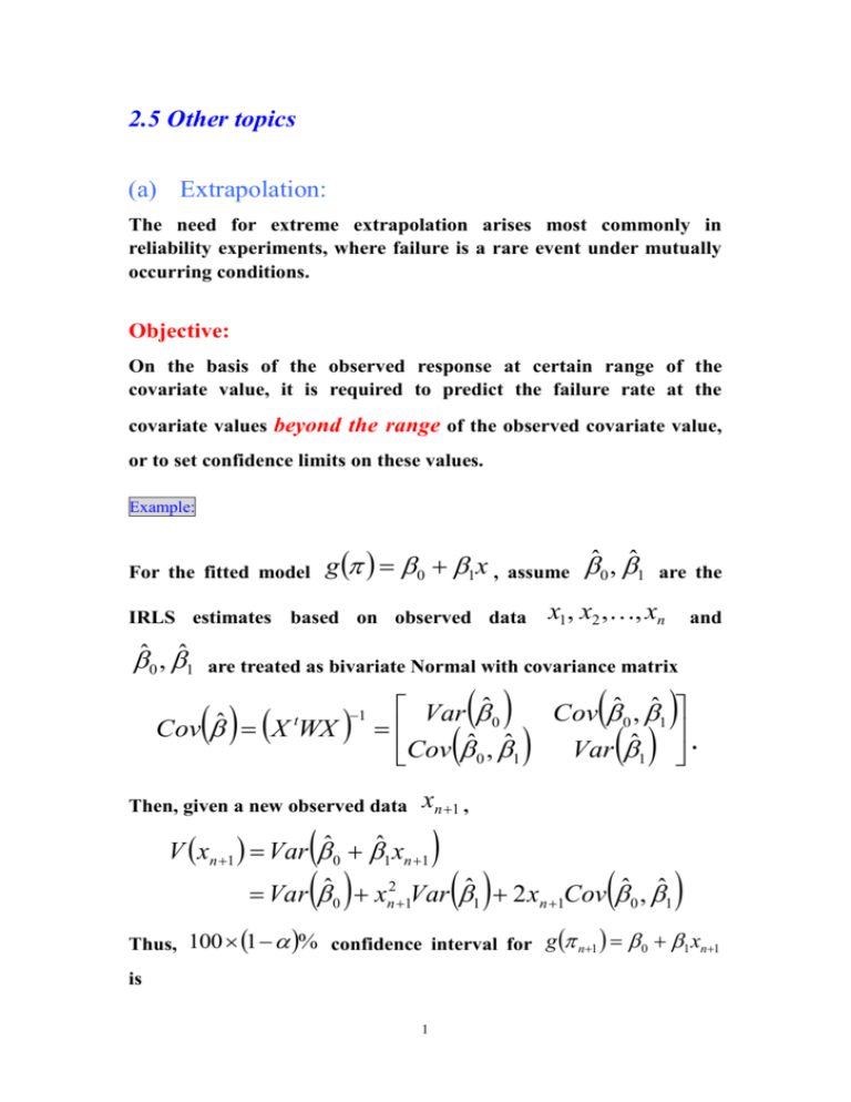
2.5 Other topics
(a) Extrapolation:
The need for extreme extrapolation arises most commonly in
reliability experiments, where failure is a rare event under mutually
occurring conditions.
Objective:
On the basis of the observed response at certain range of the
covariate value, it is required to predict the failure rate at the
covariate values beyond the range of the observed covariate value,
or to set confidence limits on these values.
Example:
For the fitted model
g     0  1x ,
assume
IRLS estimates based on observed data
ˆ0 , ˆ1
ˆ0 , ˆ1
are the
x1 , x2 ,, xn
and
are treated as bivariate Normal with covariance matrix
 
Cov ˆ  X tWX

1
Then, given a new observed data

 
 
 Var ˆ0

ˆ ˆ
Cov  0 , 1



Cov ˆ0 , ˆ1
Var ˆ1
 


.
xn 1 ,

V xn 1   Var ˆ0  ˆ1 xn 1
 Var ˆ0  xn21Var ˆ1  2 xn 1Cov ˆ0 , ˆ1
 


Thus, 100  1   % confidence interval for g  n1    0  1 xn1
is
1
ˆ0  ˆ1 xn 1  g  n 1 
 z1
V xn 1 

 g  n 1   ˆ0  ˆ1 xn 1  V xn 1 z1 , ˆ0  ˆ1 xn 1  V xn 1 z1

On the other hand, given a failure probability  0 , the 100  1   %
confidence “interval” is the set of all x0 -values satisfying
ˆ0  ˆ1 x0  g  0 
V  x0 
 z1
.
(b) Over-dispersion:
By the term “over-dispersion”, it means the variance of the response
Yi exceeds the nominal variance mi i 1   i  .
Note:
Some would maintain that over-dispersion is the norm in practice
and nominal dispersion the exception.
Note:
Over-dispersion can arise in a number of ways. The simplest and the
most common is clustering in the population.
(I) Over-dispersion for clustering:
Assume for simplicity that the cluster size is equal to k and the
sample size is equal to m. Thus, there are
m
clusters. Let
k
Z j ~ bk ,  j  be the number of positive respondents in the j’th
2
cluster. Then, the total number of positive respondents is
Y  Z1  Z 2    Z m
k
.
Assume  j is a random variable with
E j    , Var j    2 1    .
Therefore, unconditional mean and variance of Y are
 mk 
 mk

 mk



E Y   E  Z j  E  E Z j |  j   E  k j 
 j 1 
 j 1

 j 1



m
 k  E  j   k 
k
j 1
m
   m
k
and
Var Y   E Var  Y |  1 ,  ,  m   Var  E  Y |  1 ,  ,  m 
 
 
k 
k 


 mk

 mk


 E  Var Z j |  j    Var  k j 
 j 1

 j 1



 mk

m
 E  k j 1   j   k 2  2 1   
k
 j 1



3


 mE    E    k m 1   
 m    1       k m 1   
 mE  j 1   j   k 2 m 1   
2
j
j
2
2
2
2
 m 1      2 m 1     k 2 m 1   
 m 1     k  1 2 m 1   

 m 1    1  k  1 2
 m 1    2
where

 2  1  k  1 2 .
Note:
If
0   2  1 , then 1   2  k  m .
(II) Parameter estimation:
In practice, it seems unwise to rely on a specific form of
over-dispersion, particularly where the assumed form has been
chosen for mathematical convenience rather than scientific
plausibility. Assume that the effect of over dispersion is
E Y   m , Var Y    2 m 1    .
That is, the mean is unaffected but the variance is inflated by an
unknown factor

2
. Then, the method in section 2.3, (b), may
still be used as if the binomial distribution continued to apply. The
differences are the following:



1
Cov ˆ   2 X tWX ,
mi 
D y1, y2 ,, yn , ~1, ~2 ,, ~n  
 2 2n p
and
4
D y1 , y2 ,, yn , ˆ 01 , ˆ 02 ,, ˆ 0 n   D y1 , y2 ,, yn , ˆ a1 , ˆ a 2 ,, ˆ an 
2
2
tends to  1 .
The only problem left is the estimation of 
2
. There are two
possible cases:
 Replication:
Suppose for each covariate value of
xi
, several observations
 yi1 , mi1 ,  yi 2 , mi 2 ,, yir , mir  , are observed. Let
i
ri
~

i


yij
j 1
ri
 mij
.
j 1
Then,
si2
~ 2
ri

yij  mij
1
i


~ 1  
~ 
ri  1 j 1 mij
i
i
The estimate of 
2
is
n
s2 
 r
i
i 1
n
 1si2
 r
i 1
5
i
 1
.
 Absence of replication:
The estimate of 
s
2
2
1

n p
is
n

i 1
 yi
 miˆ i 
X2

miˆ i 1  ˆ i 
n p
2
Note:
If
mi  1
for each i, the estimate of 
2
based on Pearson’s
statistic does not have a close approximation of true 
6
2
.