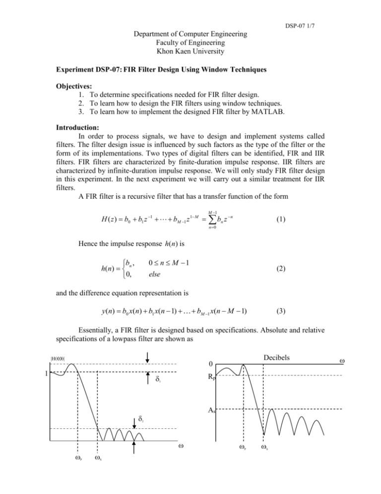
DSP-07 1/7
Department of Computer Engineering
Faculty of Engineering
Khon Kaen University
Experiment DSP-07: FIR Filter Design Using Window Techniques
Objectives:
1. To determine specifications needed for FIR filter design.
2. To learn how to design the FIR filters using window techniques.
3. To learn how to implement the designed FIR filter by MATLAB.
Introduction:
In order to process signals, we have to design and implement systems called
filters. The filter design issue is influenced by such factors as the type of the filter or the
form of its implementations. Two types of digital filters can be identified, FIR and IIR
filters. FIR filters are characterized by finite-duration impulse response. IIR filters are
characterized by infinite-duration impulse response. We will only study FIR filter design
in this experiment. In the next experiment we will carry out a similar treatment for IIR
filters.
A FIR filter is a recursive filter that has a transfer function of the form
H ( z )  b0  b1 z 1    bM 1 z 1 M 
M 1
b z
n 0
n
(1)
n
Hence the impulse response h(n) is
0  n  M 1
else
b ,
h( n)   n
0,
(2)
and the difference equation representation is
y(n)  b0 x(n)  b1 x(n  1)    bM 1 x(n  M  1)
(3)
Essentially, a FIR filter is designed based on specifications. Absolute and relative
specifications of a lowpass filter are shown as
|H()|
Decibels


Rp
1
As
2

P
S
P
S

DSP-07 2/7
where 1 is passband ripple, Rp is passband ripple in dB, 2 is stopband ripple, As is
stopband ripple in dB, p is passband edge frequency, and s is stopband edge frequency.
The parameters given in the above two specifications are obviously related by
R p  20 log 10
As  20 log 10
1  1
 0 ( 0)
1  1
2
 0 ( 1)
1  1
(4)
Note: Unit of Rp and As is decibel (dB). By the meaning of attenuation, we always have
the positive values of Rp and As.
The basic idea behind the window design is to select an appropriate window
function and an appropriate ideal filter that provides a linear-phase and causal FIR filter.
Let w(n ) and hd (n) be the window function and the impulse response of the ideal filter,
respectively. The impulse response of the designed filter can be formed by
h(n)  hd (n) w(n)
(5)
There are several window functions available. Each of those window functions
has different characteristics in both time-domain and frequency-domain. We now briefly
describe various well-known window functions.
1. Rectangular Window This is the simplest window function but provides the
worst performance from the viewpoint of stopband attenuation. It is defined by
1,
w(n)  
0,
0  n  M 1
otherwise
(6)
2. Bartlett Window Since the Gibbs phenomenon results from the fact that the
rectangular window has a sudden transition from 0 to 1 (or 1 to 0), Bartlett suggested a
more gradual transition in the form of a triangular window, which is given by
 2n
M 1,

2n
w(n)  2 
,
M

1

0,

0n
M 1
2
M 1
 n  M 1
2
otherwise
(7)
DSP-07 3/7
3. Hanning Window This is a raised cosine window given by


 2n 
 , 0  n  M 1
0.5 * 1  cos
M  1 



w(n)  
0,
otherwise

(8)
4. Hamming Window This window is similar to the Hanning window except that
it has a small amount of discontinuity and is given by

 2n 
0.54  0.46 * cos M  1 , 0  n  M  1


w(n)  
0,
otherwise

(9)
5. Blackman Window This is also similar to the previous two but contains a
second harmonic term and is given by

 2n 
 4n 
0.42  0.5 cos
  0.08 cos
, 0  n  M  1


M  1
M  1


w(n)  
0,
otherwise


(10)
Given transition width and minimum stopband attenuation of the desired filter, we can
select suitable window type and widow size based on information in Table 1.
Window Name
Rectangular
Bartlett
Hanning
Hamming
Blackman
Transition Width 
Approximate
Exact Values
4
1.8
M
M
8
6.1
M
M
8
6.2
M
M
8
6.6
M
M
12
11
M
M
Min. Stopband
Attenuation
21 dB
25 dB
44 dB
53 dB
74 dB
Table 1. Summary of commonly used window function characteristics
DSP-07 4/7
6. Kaiser window


1
 
2
2
 I 0   1   (n   ) /  
 / I0 ( ) 0  n  M 1
(11)
w(n)   


0
otherwise

where  = (M-1)/2 and I0 = the zeroth order Modified Bessel Function
If  p ,  s , R p , and As are given then the following equations are needed for
design.
Transition width  f 
Filter order M 
s   p
2
As  7.95
1
14.36f
0.1102( As  8.7),


Parameter   0.5842( As  21)0.4  0.07886( As  21),

0

(12)
As  50
21  As  50
As  21
MATLAB provides several routines to implement window functions. A brief
description of these routines is given below.
 w = boxcar(M) returns the M-point rectangular window function in array w.
 w = triang(M) returns the M-point Bartlett (triangular) window function in
array w.
 w = hanning(M) returns the M-point Hanning window function in array w.
 w = hammimg(M) returns the M-point Hamming window function in array w.
 w = blackman(M) returns the M-point Blackman window function in array w.
DSP-07 5/7
Experiment:
1. To design FIR filters based on the window technique, an ideal lowpass impulse
response hd (n) is required. Therefore it is convenient to have a simple routine that
creates hd (n) as shown below.
function hd = ideal_lp(wc, M)
% Ideal LowPass filter computation
% ---------------------------------------% [hd] = ideal_lp(wc, M)
%
hd = ideal impulse response between 0 to M-1
%
wc = cutoff frequency in radians
%
M = length of the ideal filter
%
alpha = (M-1)/2;
n = [0:1:(M-1)]
M = n – alpha + eps;
% add smallest number to avoid divide by zero
hd = sin(wc*M) ./ (pi*M);
2. To display the frequency-domain plots of digital filter, create and save the below
function, which returns the magnitude response in absolute as well as in relative dB scale,
the phase response, and the group delay response.
function [db, mag, pha, grd, w] = freqz_m(b, a)
% Modified version of freqz sunroutine
% --------------------------------------------% [db,mag,pha,grd,w] = freqz_m(b, a)
% db = Relative magnitude in dB computed over 0 to pi radians
% mag = absolute magnitude computed over 0 to pi radians
% pha = Phase response in radians over 0 to pi radians
% grd = group delay over 0 to pi radians
%
w = 501 frequency samples between 0 to pi radians
%
b = numerator polynimial of H(z)
(for FIR: b=h)
%
a = denominator polynomial of H(z) (for FIR: a=[1])
%
[H,w] = freqz(b,a,1000,’whole’);
H = (H(1:1:501))’;
w = (w(1:1:501))’;
mag = abs(H);
db = 20*log10((mag+eps)/max(mag));
pha = angle(H);
grd = grpdelay(b,a,w);
% End of function
3. With the given specifications
 p  0.3 ,  s  0.4 , R p  0.25 dB, and As  50 dB
Enter the following commands as design steps of the FIR lowpass filter using hamming
window. Save the plots
>> wp = 0.3*pi; ws = 0.4*pi;
>> tr_width = ws-wp;
>> M = ceil(6.6*pi/tr_width)+1;
>> n = [0:1:M-1];
>> wc = (ws+wp)/2;
>> hd = ideal_lp(wc,M);
>> w_ham = (hamming(M))’;
>> h = hd .* w_ham;
>> [db,mag,pha,grd,w] = freqz_m(h,[1]);
% plots
>> subplot(1,1,1)
>> subplot(2,2,1); stem(n,hd); title(‘Ideal Impulse Response’)
>>
>>
>>
>>
>>
>>
>>
>>
>>
DSP-07 6/7
axis([0 M-1 –0.1 0.3]); xlabel(‘n’); ylabel(‘hd(n)’)
subplot(2,2,2); stem(n, w_ham); title(‘Hamming Window’)
axis([0 M-1 0 1.1]); xlabel(‘n’); ylabel(‘w(n)’)
subplot(2,2,3); stem(n,h); title(‘Actual Impulse Response’);
axis([0 M-1 –0.1 0.3]); xlabel(‘n’); ylabel(‘h(n)’);
subplot(2,2,4); plot(w/pi, db); title(‘Magnitude Response in dB’);
grid
axis([0 1 –100 10]); xlabel(‘frequency in pi units’);
ylabel(‘Decibels’)
4. Find the value of M, R p , and As of the designed filter in the procedure (3)
5. Using the MATLAB function called filter, apply the filter designed in (3) to the
input signal used in the previous experiment, which saved in the file lab4sig.mat. Then
plot the input signal and the filtered output signal. Save the plot.
6. Design the FIR highpass filter using Kaiser window. Save the plots.
>> wp = 0.3*pi; ws = 0.4*pi; As = 50;
>> tr_width = (ws-wp)/(2*pi);
6.1 Write your own equation to compute the filter order M for the Kaiser window
>>
>>
>>
>>
M =
n = [0:1:M-1];
wc = (ws+wp)/2;
hd = ideal_lp(pi, M)-ideal_lp(wc,M);
6.2 Write your own equation to compute parameter  for the Kaiser window
>> beta =
6.3 Write your own equation to compute Kaiser window coefficients (see function besseli
in MATLAB for help)
>> w_kaiser =
>> h = hd .* w_kaiser;
>> [db,mag,pha,grd,w] = freqz_m(h,[1]);
% plots
>> subplot(1,1,1)
>> subplot(2,2,1); stem(n,hd); title(‘Ideal Impulse Response’)
>> axis([0 M-1 –0.1 0.3]); xlabel(‘n’); ylabel(‘hd(n)’)
>> subplot(2,2,2); stem(n, w_ham); title(‘Hamming Window’)
>> axis([0 M-1 0 1.1]); xlabel(‘n’); ylabel(‘w(n)’)
>> subplot(2,2,3); stem(n,h); title(‘Actual Impulse Response’);
>> axis([0 M-1 –0.1 0.3]); xlabel(‘n’); ylabel(‘h(n)’);
>> subplot(2,2,4); plot(w/pi, db); title(‘Magnitude Response in dB’);
>> grid
>> axis([0 1 –100 10]); xlabel(‘frequency in pi units’);
>> ylabel(‘Decibels’)
Questions:
1. Given the specifications for a digital bandpass filter as below
lower stopband edge : ω1s  0.2 ,
As  60 dB
lower passband edge : ω1 p  0.35 ,
R p  1 dB
upper passband edge :  2 p  0.65 ,
R p  1 dB
upper stopband edge :  2 s  0.8 ,
As  60 dB
1.1 Sketch the relative specifications of the filter.
1.2 Design the filter using the Blackman window.
2. What is a built-in MATLAB function that can be used to design FIR filters? Explain
how to use that function.
Nawapak Eua-anant and Rujchai Ung-arunyawee, 24 January 2549
DSP-07 7/7
Name:______________________________________________________________ID:________________
In class assignment DSP07
1. From This experiment, explain briefly advantages of FIR Filters.
2. For the rectangular, Blackman, Hamming, and Hanning windows with equal size, write down the name
of the windows in the order based on width of the main lobe of their spectrum from the narrowest to the
widest.
3. Which MATLAB commands in procedure 3 that are used to compute the number of points of the
Hamming window?
4. What knowledge do you get from this lab?