6 May 2014
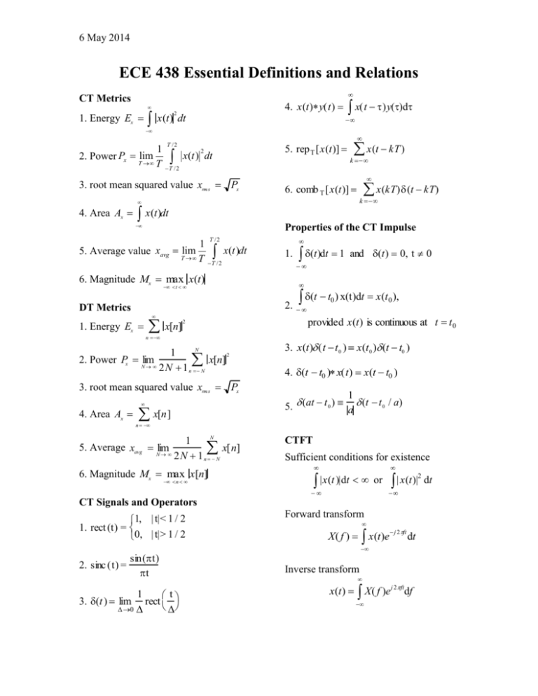
ECE 438 Essential Definitions and Relations

CT Metrics
4. x(t)y(t) 

1. Energy Ex 

2
x(t) dt
 x(t  )y()d



 x(t  kT )
1
2
x(t) dt
2. Power Px  lim

T  T
T /2
5. rep T [x(t)] 
3. root mean squared value xrm s  Px
6. comb T [x(t)] 
T /2
k 

 x(kT) (t  kT)
k 

4. Area Ax 
 x(t)dt
Properties of the CT Impulse


T /2
1
x(t)dt
T  T 
T /2
5. Average value xavg  lim
1.
6. Magnitude Mx  max x(t)
2.
1. Energy Ex 


x[n]
2
n  
N
1
2
2. Power Px  lim
x[n]

N   2N 1
n  N
3. root mean squared value xrm s  Px
4. Area Ax 

 x[n]
and (t)  0, t  0

 t  
DT Metrics
 (t)dt  1

 (t  t0 ) x(t)dt  x(t 0 ),

provided x(t) is continuous at t  t 0
3. x(t) (t t 0 )  x(t 0 ) (t  t0 )
4. (t  t0 ) x(t)  x(t  t0 )
1
5.  (at  t 0 )  a  (t  t 0 / a)
n  
N
1
x[n]

N   2N  1
n  N
5. Average xavg  lim
6. Magnitude Mx  max x[n]
 n  
CT Signals and Operators
1, | t|< 1 / 2
1. rect (t) = 
0, | t|> 1 / 2
CTFT
Sufficient conditions for existence

 |x(t )|dt  


 | x(t)|
2
or

Forward transform

X( f ) 
 x(t)e
 j 2 ft
dt

2. sinc (t) =
sin(t)
t
1
 t
3. (t )  lim rect  
 0 
 
Inverse transform

x(t) 
 X( f )e

j 2 ft
df
dt
6 May 2014
-2 -
Transform Relations
ECE 438 Essential Definitions ...
CT FT
1. rect (t)  sinc (f)
1. Linearity
CT FT
a1 x1(t)  a2 x 2 (t)  a1X1( f )  a2 X 2 ( f )
2. Scaling and shifting
t  t0 CT FT
x
 |a| X(af )e j2ft 0
 a 
j2 f 0 t
CT FT
CT FT
j2 f t
3. e 0  ( f  f 0 )
CT FT 1
4.
3. Modulation
x(t)e
CT FT
2. (t )  1 and 1  ( f )
cos(2f 0 t) 
2
{( f  f 0 )
 ( f  f 0 )}
CT FT
 X( f  f 0 )
DT Signals and Operators
4. Reciprocity
1, n  0
1. u[n] = 
0, n < 0
CT FT
X(t)  x( f )
5. Parseval

 |x(t )|
2

dt 

 | X( f )|
2
df
1,
2. [n] = 
0,

3. x[n]y[n] 
6. Initial Value
 x[n  k]y[k]
 x(t) dt


x(0) 

k 

X(0) 
n0
n0
 X( f ) df
x[n]
CT FT
x(t)y(t)  X( f )Y( f )
y[n]
4. Downsampling
y[n]  x[Dn]

7. Convolution
D
x[n]
D
y[n]
5. Upsampling
x[n / D], n / D integer - valued
y[n]  
else
 0,
8. Product
CT FT
x(t)y(t)  X ( f )Y( f )
9. Transform of periodic signal
CT FT 1
rep T [x(t)]  comb 1 [X( f )]
T
T
10. Transform of sampled signal
CT FT 1
comb T [x(t)]  rep 1 [X( f )]
T
T
Properties of the DT Impulse

1.
 [n]  1 and [n]  0, n  0
n 

2.
 [n  n0 ] x[n]  x[n0 ]
n 
3. [n  n0 ]x[n]  x[n  n0 ]
DTFT
Transform Pairs
Sufficient conditions for existence
6 May 2014


-3 
 x[n] 2  
x[n]   or
n 
n 
Forward transform
X() 
ECE 438 Essential Definitions ...

x[n]
8. Downsampling
1 D1   2k 
Y ()   X 
D k 0
D 
 x[n]e  jn
n 
Inverse transform

1
jn
x[n] 
X()e d

2 
y[n]
D
x[n]
D
y[n]
10. Upsampling
Y()  X(D)
Transform Pairs
DTFT
1. [n]  1
Transform Relations
DT FT
2. 1  2 rep2  [()]
1. Linearity
DT FT
a1 x1[n]  a2 x 2 [n]  a1X1 ()  a2 X 2 ()
DT FT
j n
3. e 0  2 rep 2  [(   0 )]
2. Shifting
DT FT
DTFT
x[n  n0 ]  X( )e  jn 0
4.
cos( 0 n) 
3. Modulation
DTFT
x[n]e j0 n  X(   0 )
4. Parseval


1
2
 x[n]  2  X() d
n 

2
 rep 2  [(   0 )  (   0 )]
 1, n  0,1,..., N  1 DTFT
x[n]  

else
 0,
X( )  psinc N ( )e j ( N 1)/2 ,
5.
sin( N / 2)
where psinc N ( ) @
sin( / 2)
5. Initial Value
X(0) 

 x[n]
n 

1
x[0] 
 X()d
2 
6. Convolution
Relation between CT and DT
1. Time Domain
xd [n]  x a (nT)
2. Frequency Domain
Xd ( d )  f s rep f s X a ( f a )
DT FT
x[n]y[n]  X()Y()
where f s 
7. Product
DT FT

1
x[n]y[n] 
 X (  )Y ()d
2 
ZT
Forward transform
1
T
fa
d f s
2
,
6 May 2014
-4 
X(z) 

ECE 438 Essential Definitions ...
DFT
x[n]z n
Forward transform
n 
N1
X[k] 
Transform Relations
ZT
a1 x1[n]  a2 x 2 [n] a1 X1 (z)  a2 X 2 (z)
2. Shifting
Inverse transform
1
x[n] 
N
ZT
x(n  n0 ) X(z)z n0
n
2. Shifting
DFT
x[n  n0 ]  X[k ]e
 j2 n 0k / N
3. Modulation
ZT
x[n]y[n] X(z)Y(z)
7. Relation to DTFT
If X ZT(z) converges for |z| 1 , then
the DTFT of x[n] exists and
XDTFT( )  XZT(z) ze j
DFT
x[n]e j2 nk0 / N  X[k  k0 ]
4. Reciprocity
DFT
X[n]  N x[k]
5. Parseval
N1

Transform Pairs
n 0
ZT
1.  [n]1, all z
ZT
1
x[n] 
N
2
N 1
 X[k ]
2
k0
6. Initial Value
N 1
1
, |z||a|
1  az1
3.  anu[n  1]
X[0]   x[n]
n 0
1
, |z||a|
1  az1
az 1
1  az 1 
2
ZT
5.  na u[n  1]
n
k 0
DFT
6. Convolution
4. n a u[n]
j2 kn /N
a1 x1[n]  a2 x 2 [n]  a1X1[k]  a2 X2 [k]
4. Multiplication by time index
ZT
d
n x[n]  z X(z)
dz
ZT
 X[k]e
1. Linearity
ZT
x[n]z0  X(z / z0 )
n
N 1
Transform Relations
3. Modulation
2. a nu[n]
 j2  kn/ N
n0
1. Linearity
ZT
 x[n]e
, | z|| a|
az
1 N 1
x[0]   X[k]
N k0
7. Periodicity
x[n  mN]  x[n] for all integers m
1
1 az 1 
2
, |z||a|
X[k  lN ]  X[k] for all integers l
6 May 2014
-5 -
8. Relation to DTFT of a finite length
sequence
Let x0 [n]  0 only for 0  n  N 1
ECE 438 Essential Definitions ...
Random Signals
1. Probability density function f X (x)
b
P{a  X  b}   f X (x)dx
DTFT
x0 [n]  X0 ( ) .
a

Define x[n] 

 x [n  mN] ,
 f X (x)dx  1
0
m 
2. Probability distribution function
FX (x)
DFT
x[n]  X[k] ,


X[k]  X0 e j2  k /N .
then
x
FX (x) 
6. Periodic convolution
DFT
7. Product
x[n]y[n] 
 f X ( )d

x[n] y[n]  X[k]Y[k]
DFT
f X (x)  0

1
X[k]  Y [k]
N
f X (x) 
dFX (x)
dx
FX ()  0 FX () 1 FX (x) is a
nondecreasing function of x
Expectation Operator

E{g(X)} 
Transform Pairs
DFT
1.
 [n], 0  n  N  1 
1. Mean g(x)  x
1, 0  k  N  1
2
2. 2nd moment g(x)  x
2
3. Variance g(x)  (x  E{X})
DFT
2.
1, 0  n  N  1 
N [k], 0  k  N  1
4. Relation between mean, 2nd moment,
and variance
 2X  E{X2} (E{X})2
DFT
3.
e j2 k 0 n /N , 0  n  N  1 
N [k - k 0 ], 0  k  N  1
DFT
cos(2  k0 n / N ), 0  n  N  1 
4.
 g(x) f X (x)dx

N
 [k - k 0 ] +  [k - (N - k0 )],
2
0  k  N 1
5.
Two Random Variables
1. Bivariate probability density function
f XY (x, y)
bd
P{a  X  b,c  Y  d}    f XY (x,y)dxdy
ac
 
  f XY (x,y)dxdy  1
f XY (x, y)  0
  
D FT
e j 0 n ,n  0,1,..., N  1 
sin (2k / N   0 )(N / 2)  j( 2  k / N   0 )( N 1 ) /2
e
sin (2k / N   0 ) / 2
2. Marginal probability density functions
f X (x) and f Y (y)
6 May 2014
-6 
f X (x) 

f XY (x, y)dy


f Y (y) 
 f XY (x, y)dx

3. Linearity of expectation
E{ag(X,Y)  bh(X,Y)}  aE{g(X,Y)} bE{h(X,Y)}
4. Correlation of X and Y
 
E{XY} 
  xyf
XY
(x, y )dxdy

5. Covariance of X and Y
 2XY  E{(X  E{X})(Y  E{Y})}
 E{XY}  E{X}E{Y}
6. Correlation coefficient of X and Y
XY 
 2XY
X Y
0 | XY |1
7. X and Y are independent if and only
if
f XY (x, y)  f X (x) f Y (y)
8. X and Y are uncorrelated if and only
if
E{XY}  E{X}E{Y}
Independence implies uncorrelatedness.
The converse is not true.
Discrete-time random signals
1. Autocorrelation function
r XX[m,m  n]  E{X[m]X[m  n]}
X[m] is wide-sense stationary if and only
if mean is constant, and autocorrelation
depends only on difference between
arguments, i.e.
E{X[n]}  X
r XX[n]  E{X[m]X[m  n]}
2. Cross-correlation function
ECE 438 Essential Definitions ...
r XY[m, m  n]  E{X[m]Y[m  n]}
X[m] and Y[m] are jointly wide-sense
stationary if and only if they are
individually wide-sense stationary and
their cross-correlation depends only on
difference between arguments, i.e.
r XY[n]  E{X[m]Y[m  n]}
3. Wide-sense stationary processes and
linear systems.
Let X[n] be wide-sense stationary, and
suppose that
Y[n]  h[n] X[n]   h[n  m]X[m] ,
m
then X[n] and Y[n] are jointly widesense stationary, and
Y   X  h[m]
m
rXY [n]  h[n]  rXX [n]
rYY [n]  h[n]  rXY [n]
Model for Speech
Our model for the speech waveform is
given by
s[n]  v[n]e[n] ,
where s[n] is the speech waveform, v[n]
is the vocal tract response that typically
contains one or more peaks
corresponding to resonant frequencies,
and e[n] is the excitation provided by
the glottis.
  [n  kP],
for a voiced phoneme,

e[n]   k
 white noise, for an unvoiced phoneme.
Here P is the pitch period in samples.
Short-Time Discrete Time Fourier
Transform (STDTFT)
Two interpretations:
6 May 2014
-7 -
1. DTFT of windowed waveform
centered at (fixed) n where w[n] is the
window function
S( , n)   s[k]w[n  k]e
ECE 438 Essential Definitions ...
that the baseband filter impulse response
h0 [n] satisfy
1 , n  0
.
h0 [n]   L
 0, n  kL
 j k
k
2. Response of narrowband filter
centered at (fixed) frequency  , after
shifting to base-band. The impulse
response of the narrowband filter
is h [n]  h0 [n]e j n . Here h0 [n] is the
impulse response of the base-band filter,
which is equivalent to the window
function w[n] in the first interpretation.
We thus have
S( , n)  h [n]  s[n]e j n
The display of the 2-D image S( ,n) as
a function of  and n is called a
spectrogram. Let N be the length of the
window function w[n] ; and let P be the
pitch period. If N ? P , the spectrogram
is narrowband. If N  P , the
spectrogram is wideband.
There are no constraints on h0 [n] for
other values of n .
2D CS Signals and Operators
1, | x| ,| y|< 1/ 2
1. rect (x, y) = 
0, | x| ,| y|> 1/ 2
2. sinc(x,y) =
1,
3. circ( x,y) = 
0
4. jinc(x,y) =
6.
A necessary and sufficient condition for
perfect reconstruction, i.e. y[n]  x[n] is
2 x 2 + y2
  f (x   , y  )g( , )d d
 
rep X,Y  f (x, y) 
7.
The output of the filter bank is formed
by summing the outputs of all L
channels
l 0

 

y[n]   yl [n]

J1  x2 + y 2
f (x, y)g(x, y) 
where
L 1
x2 + y 2  1 / 2
1
x y 
2 rect  , 
 0 
 
yl [n]  hl [n]  x[n] ,
hl [n]  h0 [n]e j 2 l n / L , l  0, ..., L  1 .
x2 + y 2  1 / 2
5.  (x, y)  lim
Modulated Filter Bank
Consider an L-channel modulated filter
bank with input x[n] and output from the
-th channel given by
sin( x) sin( y)
x
y

  f x  kX, y  lY 
k   l  
comb X,Y  f (x, y) 

8.

  f kX,lY  x  kX, y  lY 
k   l  
9. Separability
f (x, y)  g(x) h(y)
6 May 2014
-8 -
2. Scaling and shifting
x  x 0 y  y0 CSFT
f 
,

a
b 
Properties of the CS Impulse
 
   (x, y) dxdy  1
1.
ECE 438 Essential Definitions ...
 
and  (x, y)  0, (x, y)  (0,0)
|ab| F(au,bv)e  j2 (ux 0 vy0 )
3. Modulation
 
   (x  x , y  y ) f (x,y)dxdy
0
j 2 (u0 x v0 y)
0
 
 f (x0 , y0 ),
2.
provided f (x, y) is continuous
at (x,y)  (x 0 , y0 )
3.
f (x, y)e
CSFT
 F(u  u0 , v  v0 )
4. Reciprocity
CSFT
F(x, y)  f (u,v)
5. Parseval
 
 (x  x 0 , y  y0 ) f (x,y) 
 
  | f (x, y)| dxdy    | F(u,v)| dudv
2
f (x  x0 , y  y0 )
2
 

6. Initial Value
CSFT
 
Sufficient conditions for existence
 

F(0,0) 
 
| f (x, y)|dxdy  
 
 
 
x(0,0) 
  | f (x, y)| dxdy  
2
or
7. Convolution
CSFT
Forward transform
f (x, y)g(x, y)  F(u,v)G(u,v)
 
  f (x, y)e
 j2 (uxvy)
dxdy
f (x, y)g(x,y)  F(u,v)G(u,v)
Inverse transform
 
  F(u,v)e
8. Product
CSFT

f (x, y) 
  F(u,v) dudv
 
 
F(u, v) 
  f (x, y) dxdy
j2  (uxvy)
dudv

Transform Relations
1. Linearity
CSFT
a1 f 1 (x,y)  a2 f 2 (x, y) 
a1F1 (u,v)  a2 F2 (u, v)
9. Transform of doubly periodic signal
CSFT 1
rep X,Y  f (x, y) 
comb 1 1 F(u, v)
,
XY
X Y
10. Transform of sampled signal
CSFT 1
comb X,Y  f (x, y) 
rep 1 1 F(u, v)
,
XY
X Y
11. Transform of separable signal
CSFT
g(x) h(y)  G(u) H(v)
6 May 2014
-9 -
2. N roots zk , k  0, , N 1 , of a
complex constant u0 , i.e. N solutions to
zN u0  0
Transform Pairs
CSFT
1. rect (x, y)  sinc(u,v)
zk  u0
CSFT
2. circ( x,y)  jinc( u, v)
CSFT
cos2 (u0 x  v 0 y) 
CTFT
5.
1
{ (u  u0 ,v  v0 )   (u  u0 ,v  v 0 )}
2
DSFT
Forward transform
X( ,  )    x[m, n]e j (m   n )
n
Inverse transform
x[m,n] 
 
X(,  )e
2   
j(m   n )
2
dd
 
Computed Tomography
1. Radon Transform (Projection)
p (t)   f (x, y) (x cos  y sin  t)dxdy
2. Fourier Slice Theorem
P ( )   p (t)e j 2  t dt
 F( cos ,  sin  )
Miscellaneous
1. Geometric Series
N1
1 z N
 z  1 z
n 0
n
e
j 2  k u 0 / N
, k  0, ,N 1
cos(   )  cos  cos  msin  sin 
sin(2 )  2 sin  cos 
CSFT
4. e j2  (u0 x v0 y)   (u  u0 ,v  v0 )
1
1/ N
3. Trigonometric Identities
sin(   )  sin  cos   cos  sin 
CSFT
3.  (x, y)  1 and 1   (u,v)
m
ECE 438 Essential Definitions ...
cos(2 )  cos 2   sin 2 
1 1
sin 2    cos(2 )
2 2
1 1
cos 2    cos(2 )
2 2
1
sin  sin   cos(   )  cos(   )
2
1
cos  cos   cos(   )  cos(   )
2
1
sin  cos   sin(   )  sin(   )
2
1
cos  sin   sin(   )  sin(   )
2