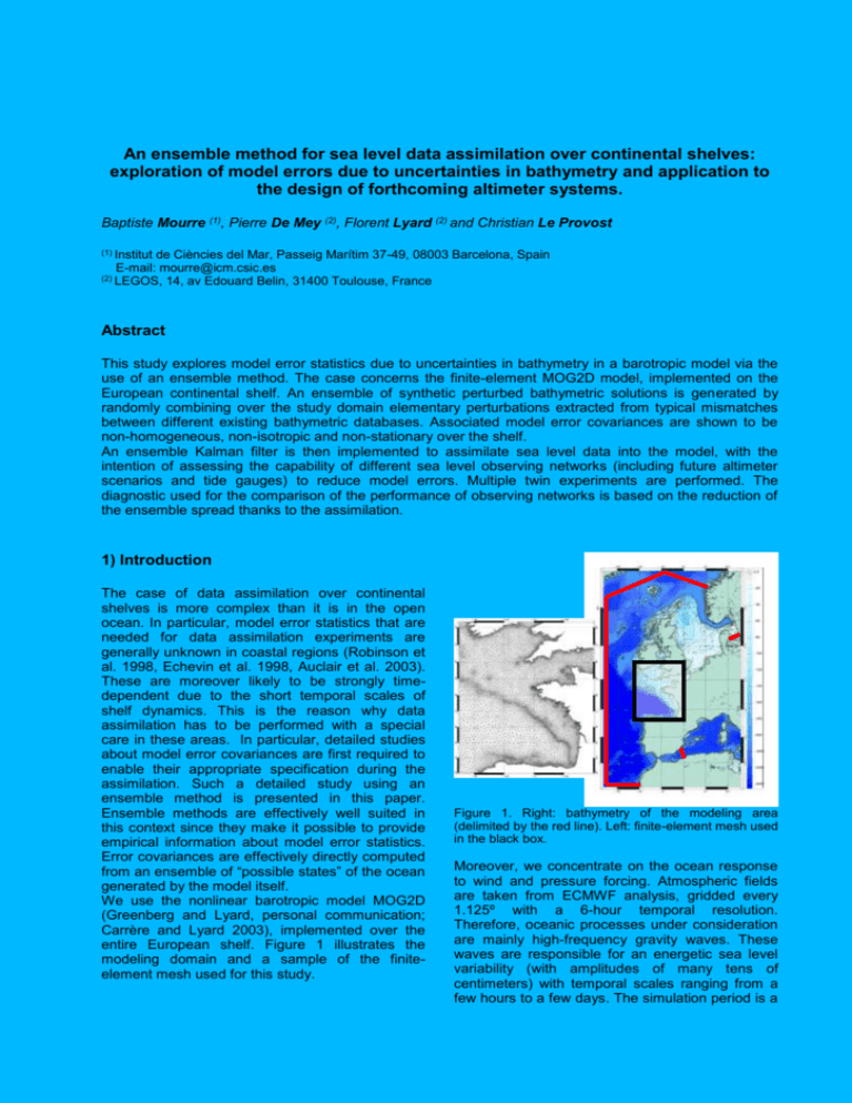
An ensemble method for sea level data assimilation over continental shelves:
exploration of model errors due to uncertainties in bathymetry and application to
the design of forthcoming altimeter systems.
Baptiste Mourre (1), Pierre De Mey (2), Florent Lyard (2) and Christian Le Provost
(1) Institut
de Ciències del Mar, Passeig Marítim 37-49, 08003 Barcelona, Spain
E-mail: mourre@icm.csic.es
(2) LEGOS, 14, av Edouard Belin, 31400 Toulouse, France
Abstract
This study explores model error statistics due to uncertainties in bathymetry in a barotropic model via the
use of an ensemble method. The case concerns the finite-element MOG2D model, implemented on the
European continental shelf. An ensemble of synthetic perturbed bathymetric solutions is generated by
randomly combining over the study domain elementary perturbations extracted from typical mismatches
between different existing bathymetric databases. Associated model error covariances are shown to be
non-homogeneous, non-isotropic and non-stationary over the shelf.
An ensemble Kalman filter is then implemented to assimilate sea level data into the model, with the
intention of assessing the capability of different sea level observing networks (including future altimeter
scenarios and tide gauges) to reduce model errors. Multiple twin experiments are performed. The
diagnostic used for the comparison of the performance of observing networks is based on the reduction of
the ensemble spread thanks to the assimilation.
1) Introduction
The case of data assimilation over continental
shelves is more complex than it is in the open
ocean. In particular, model error statistics that are
needed for data assimilation experiments are
generally unknown in coastal regions (Robinson et
al. 1998, Echevin et al. 1998, Auclair et al. 2003).
These are moreover likely to be strongly timedependent due to the short temporal scales of
shelf dynamics. This is the reason why data
assimilation has to be performed with a special
care in these areas. In particular, detailed studies
about model error covariances are first required to
enable their appropriate specification during the
assimilation. Such a detailed study using an
ensemble method is presented in this paper.
Ensemble methods are effectively well suited in
this context since they make it possible to provide
empirical information about model error statistics.
Error covariances are effectively directly computed
from an ensemble of “possible states” of the ocean
generated by the model itself.
We use the nonlinear barotropic model MOG2D
(Greenberg and Lyard, personal communication;
Carrère and Lyard 2003), implemented over the
entire European shelf. Figure 1 illustrates the
modeling domain and a sample of the finiteelement mesh used for this study.
Figure 1. Right: bathymetry of the modeling area
(delimited by the red line). Left: finite-element mesh used
in the black box.
Moreover, we concentrate on the ocean response
to wind and pressure forcing. Atmospheric fields
are taken from ECMWF analysis, gridded every
1.125º with a 6-hour temporal resolution.
Therefore, oceanic processes under consideration
are mainly high-frequency gravity waves. These
waves are responsible for an energetic sea level
variability (with amplitudes of many tens of
centimeters) with temporal scales ranging from a
few hours to a few days. The simulation period is a
25-day period from 7 to 31 December 1998.
In this context of barotropic shelf dynamics,
bathymetric uncertainties represent a potential
source of error for the model. Our insufficient
knowledge of bottom topography in most shallow
regions of the world makes the introduction of such
errors generally unavoidable. As an illustration,
figure 2 displays the RMS dispersion of gravity
wave speed estimates ( gH ) computed from five
different
bathymetric
databases
(ETOPO2,
DBDB5, TERRAINBASE, SMITH&SANDWELL
6.2, SHOM) in the Bay of Biscay and the English
Channel. This dispersion reaches values up to 60
% of the local gravity wave speed estimate next to
the coast and along the shelf break. As trapped
gravity waves essentially propagate along these
two guides, one can expect a significant impact of
these topographic uncertainties on the free surface
model. This particular impact is investigated here
in the context of data assimilation, in other words
with a focus on the associated model error
statistics.
generated by perturbing a reference bathymetric
solution (the one from the SHOM1 in our case) with
a random combination of elementary perturbations
over the study domain. These elementary
perturbations
are
extracted
from
typical
mismatches between the 5 above-mentioned
existing bathymetric databases. They are divided
into 6 types: littoral and shelf perturbations, shelf
break perturbations, deep ocean perturbations,
perturbations in straits, horizontal offsets and
vertical offsets. In concrete terms, each global
perturbation is a linear combination with random
coefficients of a random number of random shapes
of each type, applied at random locations in their
geographic domain of validity (e.g. a shelf
perturbation shape is always applied on a shelf).
The random numbers used at each step of this
procedure are taken from Gaussian distributions,
whose spreads are determined in such a way that
the final bathymetric ensemble dispersion
approaches the empirical one computed from the
sample of the 5 existing bathymetric solutions.
Then the model run over these perturbed solutions
leads to an ensemble of simulations providing
empirical information about model error statistics
and their evolution relative to this particular source
of error. Mean sea level ensemble variances over
the simulation period obtained by this approach
are illustrated in figure 3.
1
2
(%)
Figure 2. RMS dispersion of gravity wave speed
estimates ( gH ) computed from 5 different bathymetric
solutions (SHOM, SMITH&SANDWELL6.2, DBDB5,
ETOPO2, TERRAINBASE)
After the description of the shape and evolution of
these statistics in section 2, the experiments
aiming at comparing different observing networks
considering in particular forthcoming altimeter
systems are presented in section 3.
2) Model error due to uncertainties in
bathymetry
An ensemble of 100 bathymetric solutions is
Figure 3. Mean sea level ensemble variances over the
study period (cm2). The dark dashed line is the 200meter isobath.
These are not homogeneous over the shelf. The
signature of bathymetric errors on model sea level
is for instance very weak in the Bay of Biscay,
where the sea level response is very close to the
inverse barometer (i.e. static response to pressure
variations), which is not dependent on depth. On
the contrary, significant values of sea level
1
Service Hydrographique et Océanographique de la
Marine
ensemble variances are reached in areas where
the specific shelf dynamics prevails, characterized
in particular by the propagation of energetic gravity
waves which are sensitive to bathymetry. This is
the case in the Channel or along Southern North
Sea coast.
Figure 4 illustrates the time evolution of these sea
level ensemble variances at two locations on the
North Sea shelf.
They evolve very quickly,
revealing that the signature of bathymetric errors
on model sea level is not stationary at all. It is also
worth noticing that this evolution is dependent on
the location under consideration, since it strongly
depends on the oceanic processes at work in its
vicinity. These processes, transient by nature,
differ as we move over the shelf.
Point 1
Point 2
Figure 5. Domains of influence (relative to sea level
forecast) of a sea level observation at the Aberdeen tide
gauge (2.1ºW, 57.1ºN) on Dec. 17 0am (a) and Dec. 21
0am (b).
On the left panel, the size of this domain of
influence relative to the sea level correction is
around 100 km, giving an idea about the extent of
the expected correction by a single sea level
observation in such a model. The right panel
illustrates how this shape varies with the evolution
of the model state. The existence of a coastal
wave at the observation time allows for instance a
correction
that
is
stretched
alongshore.
Assimilation schemes used in these areas also
have to consider these evolving characteristics of
error covariances.
3) Design of forthcoming altimeter systems
Figure 4. Sea level ensemble variance time series at
locations 1 and 2 represented in figure 3.
Anyway, these properties of non-homogeneity and
non-stationarity of sea level model error have to be
considered in assimilation experiments that are
performed
in
such
regions.
Common
simplifications are no more valid here, and ad hoc
exploration and modeling of error statistics are
required.
We illustrate in figure 5 the domain of influence of
a single sea level observation on the North Sea
shelf, and its evolution. The domain of influence is
the area of significant correlations with the
observed variable, in other words here the area in
which the given sea level observation is likely to
make it possible to correct model sea level. Here
we arbitrarily define this domain of influence as the
area of correlations higher than 0.6.
In order to take into account the non-homogeneity,
non-stationarity and non-isotropy of model error
covariances, an ensemble Kalman filter (Evensen
2003) is implemented to assimilate sea level data
in the model. Note that we now concentrate on the
North Sea for these experiments. Multiple twin
experiments are performed to evaluate the
performance of a given observing system to
reduce model error.
In concrete terms, an
ensemble of observations is simulated from a
reference run, with random perturbations
corresponding to the observational noise. These
observations are then used to update the
ensemble of model states. Observations are
treated as random variables to avoid an
underestimation of analysis ensemble variances
(Burgers et al. 1998). The comparison of the
ensemble spread without assimilation to the one
with assimilation of data coming from a given
observing scenario finally gives insights into the
reduction of model error by the assimilation.
Figure 6 illustrates this approach in the case of a
single Jason satellite (10-day repititivity period), at
location 1. Each vertical dotted line corresponds to
an analysis, in other words to an altimeter track
crossing the North Sea shelf. Only analysis
associated with tracks coming in the vicinity (in the
sense of the domain of influence of the
observations) of the location under consideration
are efficient for the local correction (see for
instance analysis on Dec. 18 and 28).
Figure 6. Time series at point 1 of ensemble sea level
without assimilation (top), ensemble sea level with
assimilation of Jason data (middle), and ensemble sea
level variances in both cases (bottom).
We limit the presentation of the results here to the
global space-time reduction of ensemble variances
over the whole domain and time period. The
interested reader can find some illustrations of the
local reduction at a given location all over the
period of sea level ensemble variances, as well as
illustrations of the spatial distribution of the
correction at a given time in Mourre et al. (2006b).
Nevertheless, these two illustrations are shown to
be very dependent on either the location or the
time under consideration, due to the spatial nonhomogeneity and non-stationarity of ensemble
variances. By computing the space-time mean, we
get rid of such dependencies and obtain a more
robust diagnostic, leading to a single space-time
global performance score for each observing
scenario.
6,6
Jason
36,4
14,0
3 Jason
45,2
16,9
4 Jason
50,8
18,8
5 Jason
53,6
19,0
6 Jason
54,3
13,3
AltiKa3 (temp. offset)
43,9
15,4
WSOA (10-day orbit)
36,3
18,4
20 tide gauges - 6h
63,2
12,6
20 tide gauges - 12h
49,9
24,8
AltiKa3 + 20 tg - 6h
70,0
26,8
WSOA + 20 tg - 6h
0
5
Performances of constellations of Jason type
satellites interleaved in time are considered in this
histogram. It shows that the impact of additional
satellites is in our case less and less significant as
the number of satellites flying increases. Then
AltiKa3 (Verron et al. 2001, Vincent and Thouvenot
2001), a constellation of 3 satellites flying in the
Envisat 35-day orbit and interleaved in time, leads
to similar performances as a constellation of 3
Jason type satellites. WSOA (Fu 2003), which is
an interferometric instrument likely to provide data
not only at the nadir of the satellite but along a
200-km swath centered on this nadir (it uses the
10-day Jason orbit here), leads to similar
performances as two nadir satellites in terms of
sea level correction, but is better than 3 in terms of
velocity correction. The correction of velocities
indeed profits from the high spatial resolution of
such instruments. Note however that the system is
not fully controllable here, whatever observing
system is considered, since bathymetry is not
corrected in these experiments. In particular, as
the bathymetric solutions are very influent on the
calculation of model velocities, the potential
correction of barotropic velocities is by construction
naturally limited in this study.
Finally, a 20 tide gauge network distributed along
North Sea coast leads to very good global
statistical performances. The reason is that they
provide a very high temporal resolution, which is
essential in our context of high-frequency
barotropic dynamics. Concerning this network, two
assimilation frequencies are considered (6 and 12
hours), as well as the combination with some
future high-resolution altimeter systems. Such
combinations lead to the best performances in our
study. More details about these configurations and
their performances are provided in Mourre et al.
(2006b).
4) Conclusions
21,2
9,6
2 Jason
scenarios. Blue bars concern sea level ensemble
variance reduction, orange bars are relative to zonal
velocity correction (the scores concerning meridional
velocities are similar).
10
15
20
25
30
69,9
35
40
45
50
55
60
65
70
75
Figure 7. Mean space-time reductions (in %) of
ensemble variances for different sea level observing
Using an ensemble method, model error
covariances due to uncertainties in bathymetry in a
barotropic model submitted to meteorological
forcing are demonstrated to be non-homogeneous,
non-isotropic and non-stationary on the European
shelf. These characteristics have to be carefully
taken into account when dealing with data
assimilation experiments over continental shelves.
Moreover, this study shows that the spread of an
ensemble with assimilation provides a robust
diagnostic for the comparison of observational
sampling strategies. The space-time mean
reduction of ensemble variances leads to a global
performance score for each observing system.
The importance of the temporal resolution of sea
level observing systems has in particular been
highlighted in the context of our study. One
recommendation would be to operate a
combination of high-resolution altimeter systems
with tide gauges to enable the best control of the
model.
Let´s finally notice that these results are relative to
the high-frequency response of the ocean to
meteorological forcing in the presence of
bathymetric uncertainties on the North Sea shelf.
The way they could be extended, or not, to other
cases (other model, other region, other error
source) is discussed in Mourre et al (2006b).
Acknowledgements
This work has been jointly supported by CNRS
(Centre National de la Recherche Scientifique) and
CNES (Centre National d'Etudes Spatiales).
In memory of Christian Le Provost.
References
Auclair F., P. Marsaleix, and P. De Mey, 2003, Spacetime structure and dynamics of the forecast error in a
coastal circulation model of the Gulf of Lions, Dyn. of
Atm. and Oceans, 36, 309-346.
Burgers G., P. J. Van Leeuwen, and G. Evensen,
1998, Analysis scheme in the ensemble Kalman Filter.
Mon. Wea. Rev., 126, 1719-1724.
Carrère L. and F. Lyard, 2003, Modeling the barotropic
response of the global ocean to atmospheric wind and
pressure forcing - comparisons with observations.
Geophys.
Res.
Lett.,
30(6):1275,
doi:10.1029/2002GL016473.
Chelton, D. B., editor, 2001, Report of the HighResolution Ocean Topography Science Working Group
Meeting. Ref. 2001-4, Oregon State Univ., Corvallis, OR.
Echevin V., P. De Mey and G. Evensen, 2000,
Horizontal and vertical structure of the representer
functions for sea surface measurements in a coastal
circulation model. J.Phys.Oceanogr., 30:2627-2635.
Evensen, G., 2003, The Ensemble Kalman Filter:
Theoretical formulation and practical implementation,
Ocean Dyn., 53, 343-367
Fu, L. L., editor, 2003, Wide-Swath Altimetric
Measurement of Ocean Surface Topography, JPL
Publication 03-002.
Mourre B., P. De Mey, F. Lyard, and C. Le Provost,
2004, Assimilation of sea level data over continental
shelves: an ensemble method for the exploration of
model errors due to uncertainties in bathymetry, Dyn. of
Atm. and Oceans, 38,93-121.
Mourre B., L. Crosnier, and C. Le Provost, 2006a,
Real-time sea level observations and operational
oceanography, Accepted for publication in Phil. Trans.
Roy. Soc. A
Mourre B., P. De Mey, Y. Ménard, F. Lyard, and C. Le
Provost, 2006b, Relative performances of future
altimeter systems and tide gauges in controlling a model
of North Sea high frequency barotropic dynamics,
submitted to Ocean Dynamics.
Robinson A. R., P. F. J. Lermusiaux and N. Quincy
Sloan III, 1998, Data assimilation. In The Sea, Volume
10, The Global Coastal Ocean: Processes and Methods,
K.H. Brink and A.R. Robinson, eds. Wiley, New York,
Chap 20.
Smith W.H.F. and D.T. Sandwell, 1997, Global seafloor
topography from satellite altimetry and ship depth
soundings. Science 277, 1957-1962.
Verron J., P. Bahurel, and P. Vincent, 2001, AltiKa :
étude de la circulation mésoéchelle par altimétrie en
bande Ka sur micro-satellite. Research Proposal to
Cnes.
Vincent P., and E. Thouvenot, 2001, Status of Ka-band
altimetry studies. In Report of the High-Resolution
Ocean Topography Science Working Group Meeting.,
editor D.Chelton, Ref. 2001-4, pp 179-189, Oregon State
Univ., Corvallis, OR