Chapter 07 - Qualitative Variables and Non-Linearities in Multiple Linear Regression Analysis
CHAPTER 7
Answers to End of Chapter Problems
7.1
a. First I would advise the Polk University not to focus too much on the R-squared
and standard error. Regression models should be built using economic theory and by
looking at other studies, not by trying to maximize R-squared or by trying to minimize
the standard error.
b. This would add two new variables.
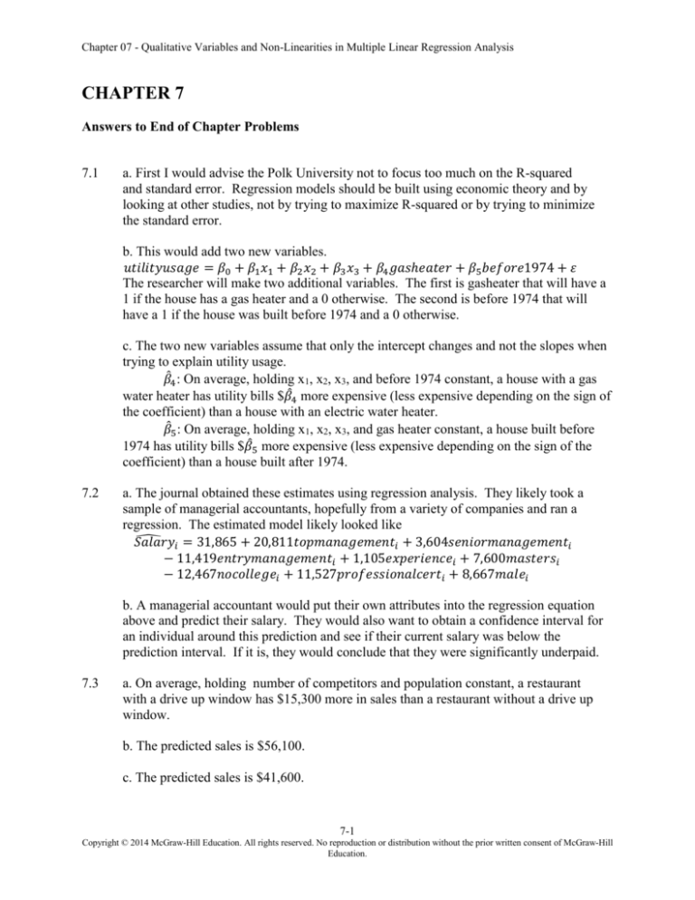
𝑢𝑡𝑖𝑙𝑖𝑡𝑦𝑢𝑠𝑎𝑔𝑒 = 𝛽0 + 𝛽1 𝑥1 + 𝛽2 𝑥2 + 𝛽3 𝑥3 + 𝛽4 𝑔𝑎𝑠ℎ𝑒𝑎𝑡𝑒𝑟 + 𝛽5 𝑏𝑒𝑓𝑜𝑟𝑒1974 + 𝜀
The researcher will make two additional variables. The first is gasheater that will have a
1 if the house has a gas heater and a 0 otherwise. The second is before 1974 that will
have a 1 if the house was built before 1974 and a 0 otherwise.
c. The two new variables assume that only the intercept changes and not the slopes when
trying to explain utility usage.
𝛽̂4 : On average, holding x1, x2, x3, and before 1974 constant, a house with a gas
water heater has utility bills $𝛽̂4 more expensive (less expensive depending on the sign of
the coefficient) than a house with an electric water heater.
𝛽̂5: On average, holding x1, x2, x3, and gas heater constant, a house built before
1974 has utility bills $𝛽̂5 more expensive (less expensive depending on the sign of the
coefficient) than a house built after 1974.
7.2
a. The journal obtained these estimates using regression analysis. They likely took a
sample of managerial accountants, hopefully from a variety of companies and ran a
regression. The estimated model likely looked like
̂ 𝑖 = 31,865 + 20,811𝑡𝑜𝑝𝑚𝑎𝑛𝑎𝑔𝑒𝑚𝑒𝑛𝑡𝑖 + 3,604𝑠𝑒𝑛𝑖𝑜𝑟𝑚𝑎𝑛𝑎𝑔𝑒𝑚𝑒𝑛𝑡𝑖
𝑆𝑎𝑙𝑎𝑟𝑦
− 11,419𝑒𝑛𝑡𝑟𝑦𝑚𝑎𝑛𝑎𝑔𝑒𝑚𝑒𝑛𝑡𝑖 + 1,105𝑒𝑥𝑝𝑒𝑟𝑖𝑒𝑛𝑐𝑒𝑖 + 7,600𝑚𝑎𝑠𝑡𝑒𝑟𝑠𝑖
− 12,467𝑛𝑜𝑐𝑜𝑙𝑙𝑒𝑔𝑒𝑖 + 11,527𝑝𝑟𝑜𝑓𝑒𝑠𝑠𝑖𝑜𝑛𝑎𝑙𝑐𝑒𝑟𝑡𝑖 + 8,667𝑚𝑎𝑙𝑒𝑖
b. A managerial accountant would put their own attributes into the regression equation
above and predict their salary. They would also want to obtain a confidence interval for
an individual around this prediction and see if their current salary was below the
prediction interval. If it is, they would conclude that they were significantly underpaid.
7.3
a. On average, holding number of competitors and population constant, a restaurant
with a drive up window has $15,300 more in sales than a restaurant without a drive up
window.
b. The predicted sales is $56,100.
c. The predicted sales is $41,600.
7-1
Copyright © 2014 McGraw-Hill Education. All rights reserved. No reproduction or distribution without the prior written consent of McGraw-Hill
Education.
Chapter 07 - Qualitative Variables and Non-Linearities in Multiple Linear Regression Analysis
7.4
a.
Hypothesis:
𝐻0 : 𝛽1 = 0 no discrimination
𝐻1 : 𝛽1 ≠ 0 discrimination
Test Statistic
t-statistic = -2.2/1= -2.2.
Rejection Rule
Reject H0 if the |t-stat| > 1.96.
Rejection Rule
Because 2.2 > 1.96 we reject H0 and conclude that males are paid
statistically less than females. Females, on average, are paid $2,200 more
than males.
b. Linear in the parameters, simple random sampling, no perfect
multicollinearity, E(ε)=0, and the zero conditional mean assumption holds.
We are also assuming that the model is homoskedastic because otherwise
the standard errors are wrong.
c. On average, male full professors are paid $18,400 more than male
assistant professors. (notice that -2.2 is subtracted for both so the effect of
that difference drops away).
d. Model (1) suffers from perfect multicollinearity because male and
female are both in the model with an intercept and all three options for
professors are in the model as well.
Model (1) cannot be estimated.
Model (2) is odd because there is no intercept but this also means that both
male and female can be in the model together. They should also add DA
into the model but with an intercept, the assumption E(ε)=0 is violated.
Neither of the initial models are superior than the initial model.
e. This model does not control for years of experience, number of
publications, different departments, if the faculty member holds an
administrative position, etc. Because these factors are omitted and also
related to the variables in the model, the estimates are biased. Therefore
the finding the discrimination exists should not be trusted because these
results are on average, wrong.
7.5
a. On average, holding the other factors in the model constant, if a person
ages by one year, their salary increases by .40762*($1000) or $407.62.
b. Hypothesis:
𝐻0 : 𝛽1 = 0
𝐻1 : 𝛽1 ≠ 0
Test Statistic
t-statistic = 0.40787/0.1027= 3.9695.
7-2
Copyright © 2014 McGraw-Hill Education. All rights reserved. No reproduction or distribution without the prior written consent of McGraw-Hill
Education.
Chapter 07 - Qualitative Variables and Non-Linearities in Multiple Linear Regression Analysis
Rejection Rule
Reject H0 if the |t-stat| > 2.
Rejection Rule
Because 3.9695 > 2 we reject H0 and conclude that age is statistically
significant at the 5% level.
c. The results from regression (1) and (2) are different because once the
other variables are controlled for in regression (2) the effect of age is no
longer statistically significant.
d. Hypothesis:
𝐻0 : 𝛽2 = 𝛽3 = 𝛽4 = 𝛽5 = 𝛽6 = 𝛽7 = 0
𝐻1 : 𝑎𝑡 𝑙𝑒𝑎𝑠𝑡 𝑜𝑛𝑒 𝛽𝑖 𝑖𝑠 𝑛𝑜𝑡 𝑒𝑞𝑢𝑎𝑙 𝑡𝑜 0
Test statistic:
(5207.7 − 2549.9)/6
𝐹 − 𝑠𝑡𝑎𝑡 =
= 12.50778
(2549.9)/(80 − 8)
Critical Value is 𝐹𝛼,𝑞,𝑛−𝑘−1 = 𝐹0.05,6,72 = 2.227
Rejection Rule:
Reject H0 if F-stat > 2.227.
Decision:
Because 12.51 < 2.227 we reject H0 and conclude that model (2) is preferable at a 5%
significance level.
e. Marginal effect of −57.737 + 2.9376 𝐴𝑔𝑒𝑖 − 0.0317𝐴𝑔𝑒𝑆𝑞𝑢𝑎𝑟𝑒𝑑𝑖 −
0.0317𝑒𝑥𝑝𝑒𝑟𝑖𝑒𝑛𝑐𝑒𝑖 .
7.6
a. Set male=0 in the data set and female = 0.
𝑠𝑎𝑙𝑎𝑟𝑦 = 𝛽0 + 𝛽1 𝑚𝑎𝑙𝑒 + 𝛽2 𝑒𝑑𝑢𝑐𝑎𝑡𝑖𝑜𝑛 + 𝜀
𝛽1 interpretation: On average, holding education constant, if a person is male then their
salary on average is 𝛽1 higher (or lower depending on the sign) than females.
𝛽2 interpretation: On average, holding male constant, if a person gets one more year of
education then salary increases by 𝛽2 dollars. Note that this effect is the same between
males and females.
b. Now interact education and male
𝑠𝑎𝑙𝑎𝑟𝑦 = 𝛽0 + 𝛽1 𝑚𝑎𝑙𝑒 + 𝛽2 𝑒𝑑𝑢𝑐𝑎𝑡𝑖𝑜𝑛 + 𝛽3 (𝑚𝑎𝑙𝑒)(𝑒𝑑𝑢𝑐𝑎𝑡𝑖𝑜𝑛) + 𝜀
𝛽1 interpretation: On average, holding education constant, if a person is male then their
salary on average is 𝛽1 higher (or lower depending on the sign) than females.
𝛽2 interpretation: On average, for men, if a man gets one more year of education then
salary increases by 𝛽2 dollars. 𝛽2 + 𝛽3 interpretation: On average, for women, if a
women gets one more year of education then salary increases by 𝛽2 + 𝛽3 dollars. 𝛽3 is
the difference in slopes between men and women.
c.
7-3
Copyright © 2014 McGraw-Hill Education. All rights reserved. No reproduction or distribution without the prior written consent of McGraw-Hill
Education.
Chapter 07 - Qualitative Variables and Non-Linearities in Multiple Linear Regression Analysis
7.7
a. On average, holding other independent variables constant, if a faculty member has
moved their salary is 11.34% higher relative to those who have not moved. This variable
is statistically significant.
On average, holding other independent variables constant, if a faculty member gets one
more year of experience then their salary is (1.13% - 0.03%experience) higher relative to
those who have not moved. This variable is statistically significant.
On average, holding other independent variables constant, if a faculty member is a male
their salary is 0.66% higher relative to a female. This variable is statistically
insignificant.
On average, holding other independent variables constant, if a faculty member has one
more top 5 article their salary increases by 3.57% higher. This variable is statistically
significant.
b. After controlling for moved and the other independent variables, on average, if a
faculty member has moved to California their salary is 12.71% higher relative to those
who haven’t moved to California. This variable is statistically significant.
After controlling for moved and the other independent variables, on average, if a faculty
member has moved from California their salary is 12.65% higher relative to those who
haven’t moved from California. This variable is statistically significant.
c. Hypothesis:
𝐻0 : 𝛽3 = 𝛽4 = 𝛽5 = 𝛽6 = 0
𝐻1 : 𝑎𝑡 𝑙𝑒𝑎𝑠𝑡 𝑜𝑛𝑒 𝛽𝑖 𝑎𝑏𝑜𝑣𝑒 𝑖𝑠 𝑛𝑜𝑡 𝑒𝑞𝑢𝑎𝑙 𝑡𝑜 0
Test Statistic
(.5025 − .4794)/4
0.262
=
= 532.95
(1 − .5025)/(1024 − 12) 0.00049
Rejection Rule
Reject H0 if the F-stat > 2.463.
Rejection Rule
𝐹 − 𝑠𝑡𝑎𝑡 =
7-4
Copyright © 2014 McGraw-Hill Education. All rights reserved. No reproduction or distribution without the prior written consent of McGraw-Hill
Education.
Chapter 07 - Qualitative Variables and Non-Linearities in Multiple Linear Regression Analysis
Because 532.95> 2.463 we reject H0 and conclude that model (2) is
statistically preferred to model (1).
d. 0.0115 -0.0003experience = 0 or where experience is equal to 38.33.
Given that this is a very long career, most faculty members will never hit
the point where salaries hit diminishing returns.
e. Using model (2), I would advise a faculty member to move as often as
possible, move both to and from California, get more experience, and
publish as many top 5 articles as possible.
Answers to End of Chapter Exercises
E7.1. a.
̂
𝐺𝑃𝐴𝑖 = 𝛽̂0 + 𝛽̂1 𝐻𝑜𝑢𝑟𝑠 𝑆𝑡𝑢𝑑𝑖𝑒𝑑𝑖 + 𝛽̂2 𝐻𝑜𝑢𝑟𝑠 𝑆𝑡𝑢𝑑𝑖𝑒𝑑 𝑆𝑞𝑢𝑎𝑟𝑒𝑑𝑖
̂ 𝑖 = 2.6576 + 0.0455𝐻𝑜𝑢𝑟𝑠 𝑆𝑡𝑢𝑑𝑖𝑒𝑑𝑖 − 0.0003𝐻𝑜𝑢𝑟𝑠 𝑆𝑡𝑢𝑑𝑖𝑒𝑑 𝑆𝑞𝑢𝑎𝑟𝑒𝑑𝑖
𝐺𝑃𝐴
Not surprisingly, GPA goes up initially as hours studied increases but there are
diminishing returns to hours studied that can be see through the negative sign on the
hours studied squared term. Because there is a quadratic effect, the effect that hours
studied has on GPA is dependent on the value of hours studied. If hours studied is 4, then
the marginal effect on GPA is
7-5
Copyright © 2014 McGraw-Hill Education. All rights reserved. No reproduction or distribution without the prior written consent of McGraw-Hill
Education.
Chapter 07 - Qualitative Variables and Non-Linearities in Multiple Linear Regression Analysis
0.0455 − (2)0.0003(3) = 0.0437 or as hours studied goes from 3 to 4 the impact on
GPA is 0.0437 points. If hours studied is 10, then the marginal effect on GPA is
0.0455 − (2)0.0003(9) = 0.0401 or as hours studied goes from 9 to 10 the impact on
GPA is 0.0401 points.
The hours studied squared term is statistically significant at the 1% level because the pvalue of 0.0019 is less than 0.01.
b. To find where hours studied reaches a maximum (or where diminishing marginal
returns sets in) set 0.0455 − 0.0003(2)𝐻𝑜𝑢𝑟𝑠 𝑆𝑡𝑢𝑑𝑖𝑒𝑑 𝑆𝑞𝑢𝑎𝑟𝑒𝑑𝑖 = 0 or when hours
studied is 75.83.
c.
Looking through the p-values, work is only statistically significant at the 10% level (not
the 5% level) and male is statistically insignificant with a p-value of 0.391. The rest of
the independent variables are statistically significant at the 5% level. To increase GPA, a
student should study more but play fewer video games and text less.
The marginal effect of hours studied is now
7-6
Copyright © 2014 McGraw-Hill Education. All rights reserved. No reproduction or distribution without the prior written consent of McGraw-Hill
Education.
Chapter 07 - Qualitative Variables and Non-Linearities in Multiple Linear Regression Analysis
0.0254 − (2)0.0002 𝐻𝑜𝑢𝑟𝑠 𝑆𝑡𝑢𝑑𝑖𝑒𝑑 𝑆𝑞𝑢𝑎𝑟𝑒𝑑𝑖 . Using the same values as before, if
hours studied is 4, then the marginal effect on GPA is
0.0254 − (2)0.0002(3) = 0.0242 or as hours studied goes from 3 to 4 the impact on
GPA is 0.0242 points. If hours studied is 10, then the marginal effect on GPA is
0.0254 − (2)0.0002(9) = 0.0218 or as hours studied goes from 9 to 10 the impact on
GPA is 0.0218 points. This function now reaches a maximum at 63.5 hours studied.
E7.2
Correlations of Annual Salary with each of the independent variables.
Salary
Female
Age
Prior Exper
-0.17704 0.9089800 0.668817843
Beta Exper
Education
0.817984548 0.649821656
Age has the strongest positive linear relationship with salary. This is a typical in labor
economics.
Female has the weakest relationship with annual salary. It is interesting that the linear
relationship between female and salary is negative suggesting that females may suffer
from discrimination at Beta.
Except for possibly Female, all the explanatory variables have a strong linear relationship
with salary.
E7.3 a.
̂
𝑃𝐶𝑇𝑖 = 𝛽̂0 + 𝛽̂1 𝐹𝐺%𝑖
̂𝑖 = −1.22 + 3.9576 𝐹𝐺%𝑖
𝑃𝐶𝑇
7-7
Copyright © 2014 McGraw-Hill Education. All rights reserved. No reproduction or distribution without the prior written consent of McGraw-Hill
Education.
Chapter 07 - Qualitative Variables and Non-Linearities in Multiple Linear Regression Analysis
b. Intercept: On average, if field goal percentage is equal to 0 then the estimated value of
proportion of games won is -1.22.
FG%: On average, if the proportion of field goals by 1% then the proportion of games
won increases by 3.95%.
c.
̂𝑖 = 𝛽̂0 + 𝛽̂1 𝐹𝐺%𝑖 + 𝛽̂2 𝑂𝑝𝑝3𝑝𝑡%𝑖 + 𝛽̂3 𝑂𝑝𝑝𝑇𝑂𝑖
𝑃𝐶𝑇
̂𝑖 = −1.235 + 4.8166 𝐹𝐺%𝑖 − 2.5895 𝑂𝑝𝑝3𝑝𝑡%𝑖 + 0.0344𝑂𝑝𝑝𝑇𝑂𝑖
𝑃𝐶𝑇
d. These results imply that for a team to increase the proportion of games won, they
should increase their field goal percentage, decrease the opponents three point percentage
and increase the number of turnovers made by the opponent.
e.
̂𝑖 = −1.235 + 4.8166 (. 45) − 2.5895 (.34) + 0.0344(17)
𝑃𝐶𝑇
̂𝑖 = 0.6377 or the team is predicted to win 63.77% of their games.
𝑃𝐶𝑇
f. The estimated regression equation does seem to provide a fairly good fit. The Rsquared is 56.38% and the standard error is 0.097. There are likely other factors that
explain winning percentage but this model looks to do relatively well.
g. Hypothesis:
𝐻0 : 𝛽1 = 𝛽2 = 𝛽3 = 0
𝐻1 : 𝑎𝑡 𝑙𝑒𝑎𝑠𝑡 𝑜𝑛𝑒 𝛽𝑖 𝑖𝑠 𝑛𝑜𝑡 𝑒𝑞𝑢𝑎𝑙 𝑡𝑜 0
Test Statistic
F-statistic = 10.77 and the p-value of the F-test is 9.9443E-05.
7-8
Copyright © 2014 McGraw-Hill Education. All rights reserved. No reproduction or distribution without the prior written consent of McGraw-Hill
Education.
Chapter 07 - Qualitative Variables and Non-Linearities in Multiple Linear Regression Analysis
Rejection Rule
Reject H0 if the p-value < 0.05.
Rejection Rule
Because 9.9443E-05< 0.05 we reject H0 and conclude that at least one of
number of FG%, Opp 3 pt%, or Opp TO explains PCT at the 5% level.
h. Using the p-values to perform the t-test, all of p-values are less than 5% and therefore
in each case the null hypothesis of no relationship is reject and all three independent
variables are statistically significant at the 5% level.
E7.4 a.
7-9
Copyright © 2014 McGraw-Hill Education. All rights reserved. No reproduction or distribution without the prior written consent of McGraw-Hill
Education.
Chapter 07 - Qualitative Variables and Non-Linearities in Multiple Linear Regression Analysis
b.
c. Hypothesis:
𝐻0 : 𝛽1 = 𝛽2 = 𝛽3 = 0
𝐻1 : 𝑎𝑡 𝑙𝑒𝑎𝑠𝑡 𝑜𝑛𝑒 𝛽𝑖 𝑖𝑠 𝑛𝑜𝑡 𝑒𝑞𝑢𝑎𝑙 𝑡𝑜 0
Test Statistic
F-statistic = 6.34 and the p-value of the F-test is 0.0031.
Rejection Rule
Reject H0 if the p-value < 0.05.
Rejection Rule
Because 0.0031< 0.05 we reject H0 and conclude that at least one of
number of weight, speed and position explains Rating at the 5% level.
d. The R-squared is 47.55%, which is high for cross sectional data and all
of the coefficient estimates are statistically significant. There are likely
other factors that also affect rating that are omitted.
e. Yes. The p-value on guard is 0.019, which is certainly less than 5%.
f.
̂ 𝑖 = 11.9556 + 0.022 𝑊𝑒𝑖𝑔ℎ𝑡𝑖 − 2.278 𝑆𝑝𝑒𝑒𝑑𝑖 − .7324𝐺𝑢𝑎𝑟𝑑𝑖
𝑅𝑎𝑡𝑖𝑛𝑔
̂ 𝑖 = 11.9556 + 0.022 (300) − 2.278 (5.1) − 0.7324(0)
𝑅𝑎𝑡𝑖𝑛𝑔
̂ 𝑖 = 6.99
𝑅𝑎𝑡𝑖𝑛𝑔
This player is just between starting and making the team as backup.
7-10
Copyright © 2014 McGraw-Hill Education. All rights reserved. No reproduction or distribution without the prior written consent of McGraw-Hill
Education.
Chapter 07 - Qualitative Variables and Non-Linearities in Multiple Linear Regression Analysis
E7.5
a.
̂
𝐻𝑜𝑢𝑠𝑖𝑛𝑔𝑃𝑟𝑖𝑐𝑒
𝑖 = −141,534.7 + 573.124𝑆𝑞𝐹𝑒𝑒𝑡𝑖 − 118,287.55𝐵𝑒𝑑𝑟𝑜𝑜𝑚𝑠𝑖
+32,007.71𝐵𝑎𝑡ℎ𝑟𝑜𝑜𝑚𝑠𝑖 + 9.56𝐿𝑜𝑡𝑆𝑖𝑧𝑒𝑖 − 195,986.59𝑃𝑜𝑜𝑙𝑖
Square Feet: On average, holding bedrooms, bathrooms, lot size, and pool constant, if a
house increases by 1 square foot then the price increases by $573.12. This is statistically
significant at the 5% level because the p-value of 1.93E-13 < 0.05.
Bedrooms: On average, holding square feet, bathrooms, lot size, and pool constant, if
the number of bedrooms in a house increases by 1 then the price drops by $118,287.55.
This is statistically significant at the 5% level because the p-value of 0.007 < 0.05. This
is a counter intuitive finding as you would expect if the number of bedrooms increases
then the price of a house would increase as well (instead of decrease).
Bathrooms: On average, holding square feet, bedrooms, lot size, and pool constant, if
the number of bedrooms in a house increases by 1 then the price drops by $118,287.55.
This is statistically insignificant at the 5% level because the p-value of 0.5635 > 0.05.
This is a counter intuitive finding as you would expect the number of bathrooms to be
statistically significant.
Lot Size: On average, holding square feet, bedrooms, bathrooms, and pool constant, if a
the lot size increases by 1 square foot then the price increases by $9.56. This is
statistically insignificant at the 5% level because the p-value of 0.2462 > 0.05.
7-11
Copyright © 2014 McGraw-Hill Education. All rights reserved. No reproduction or distribution without the prior written consent of McGraw-Hill
Education.
Chapter 07 - Qualitative Variables and Non-Linearities in Multiple Linear Regression Analysis
Pool: On average, holding square feet, bedrooms, bathrooms, and lot size constant, a
house with a pool costs $195,986.59 less than a house without a pool. This is
statistically insignificant at the 5% level because the p-value of 0.064 > 0.05 (but it is
significant at the 10% level). This is also a counter intuitive result because we would
expect that a house with a pool would be more valuable.
b.
Now the statistically significant variables at the 5% level are square feet, bedrooms,
bedrooms*lotsize, and pool. Lot size is statistically significant at the 10% level.
Marginal effect of LotSize:
−63.5 + 18 𝐵𝑒𝑑𝑟𝑜𝑜𝑚𝑠𝑖
Notice this is marginal effect changes as the number of bedrooms change.
Marginal effect of Bedrooms:
−232,382 + 18 𝐿𝑜𝑡𝑠𝑖𝑧𝑒𝑖
Notice this is marginal effect changes as the lot size changes.
If instead you interact bedrooms and square footage then the results are
7-12
Copyright © 2014 McGraw-Hill Education. All rights reserved. No reproduction or distribution without the prior written consent of McGraw-Hill
Education.
Chapter 07 - Qualitative Variables and Non-Linearities in Multiple Linear Regression Analysis
Now the statistically significant variables at the 5% level are bedrooms, square
feet*bedrooms, and pool.
Marginal effect of Square Feet:
95.41 + 124.92 𝐵𝑒𝑑𝑟𝑜𝑜𝑚𝑠𝑖
Notice this is marginal effect changes as the number of bedrooms change.
Marginal effect of Bedrooms:
−340,050.44 + 124.92 𝑆𝑞𝑢𝑎𝑟𝑒𝐹𝑒𝑒𝑡𝑖
Notice this is marginal effect changes as square feet changes.
7-13
Copyright © 2014 McGraw-Hill Education. All rights reserved. No reproduction or distribution without the prior written consent of McGraw-Hill
Education.
Chapter 07 - Qualitative Variables and Non-Linearities in Multiple Linear Regression Analysis
E7.6
a.
̂
ln(𝐻𝑜𝑢𝑠𝑖𝑛𝑔𝑃𝑟𝑖𝑐𝑒)
𝑖 = 12.15 + 0.0007𝑆𝑞𝐹𝑒𝑒𝑡𝑖 − 0.063𝐵𝑒𝑑𝑟𝑜𝑜𝑚𝑠𝑖
− 0.000004 𝐿𝑜𝑡𝑆𝑖𝑧𝑒𝑖 − 0.175 𝑃𝑜𝑜𝑙𝑖
Square Feet: On average, holding bedrooms, bathrooms, lot size, and pool constant, if
the square feet of a house increases by 1 square foot then the price increases by .07%.
This is statistically significant at the 5% level because the p-value of 8.45E-13 < 0.05.
Bedrooms: On average, holding square feet, bathrooms, lot size, and pool constant, if
the number of bedrooms in a house increases by 1 then the price drops by 6.3%. This is
statistically insignificant at the 5% level because the p-value of 0.18 > 0.05.
Lot Size: On average, holding square feet, bedrooms, bathrooms, and pool constant, if
the lot size increases by 1 square foot then the price decreases by 0.0004%. This is
statistically insignificant at the 5% level because the p-value of 0.674 > 0.05.
Pool: On average, holding square feet, bedrooms, bathrooms, and lot size constant, a
house with a pool costs 17.4% less than a house without a pool. This is statistically
insignificant at the 5% level because the p-value of 0.13 > 0.05.
7-14
Copyright © 2014 McGraw-Hill Education. All rights reserved. No reproduction or distribution without the prior written consent of McGraw-Hill
Education.
Chapter 07 - Qualitative Variables and Non-Linearities in Multiple Linear Regression Analysis
b.
̂
ln(𝐻𝑜𝑢𝑠𝑖𝑛𝑔𝑃𝑟𝑖𝑐𝑒)
𝑖 = 3.58 + 1.33 ln(𝑆𝑞𝐹𝑒𝑒𝑡)𝑖 − 0.1034 𝐵𝑒𝑑𝑟𝑜𝑜𝑚𝑠𝑖
+ 0.000008 𝐿𝑜𝑡𝑆𝑖𝑧𝑒𝑖 − 0.1245 𝑃𝑜𝑜𝑙𝑖
Square Feet: On average, holding bedrooms, bathrooms, lot size, and pool constant, if
the square feet of a house increases by 1% then the price increases by 1.33%. This is
statistically significant at the 5% level because the p-value of 2.22E-21 < 0.05.
Bedrooms: On average, holding square feet, bathrooms, lot size, and pool constant, if
the number of bedrooms in a house increases by 1 then the price drops by 10.34%. This
is statistically significant at the 5% level because the p-value of 0.047 < 0.05.
Lot Size: On average, holding square feet, bedrooms, bathrooms, and pool constant, if
the lot size increases by 1 square foot then the price decreases by 0.0008%. This is
statistically insignificant at the 5% level because the p-value of 0.377 > 0.05.
Pool: On average, holding square feet, bedrooms, bathrooms, and lot size constant, a
house with a pool costs 12.45% less than a house without a pool. This is statistically
insignificant at the 5% level because the p-value of 0.30 > 0.05.
7-15
Copyright © 2014 McGraw-Hill Education. All rights reserved. No reproduction or distribution without the prior written consent of McGraw-Hill
Education.
Chapter 07 - Qualitative Variables and Non-Linearities in Multiple Linear Regression Analysis
E7.7
Looking over the results, the p-value for the F-test (0.3322) is greater than 0.05, which
implies that all independent variables are jointly insignificant. Looking over the t-tests
for individual significant, only sequel is statistically significant at the 10% level and none
of the variables are statistically significant at the 5% level. Perform an F-test will all
variables except for sequel dropped out of the model yields a restricted regression of
7-16
Copyright © 2014 McGraw-Hill Education. All rights reserved. No reproduction or distribution without the prior written consent of McGraw-Hill
Education.
Chapter 07 - Qualitative Variables and Non-Linearities in Multiple Linear Regression Analysis
Now sequel is statistically significant at the 5% level.
Hypothesis:
𝐻0 : 𝛽1 = 𝛽2 = 𝛽3 = 𝛽4 = 𝛽5 = 𝛽7 = 𝛽8 = 0
𝐻1 : 𝑎𝑡 𝑙𝑒𝑎𝑠𝑡 𝑜𝑛𝑒 𝛽𝑖 𝑖𝑠 𝑛𝑜𝑡 𝑒𝑞𝑢𝑎𝑙 𝑡𝑜 0
Test statistic:
(3.6731𝐸 + 12 − 3.31375𝐸 + 12)/7
𝐹 − 𝑠𝑡𝑎𝑡 =
= 0.6817
(3.31375𝐸 + 12)/44
Critical Value is 𝐹𝛼,𝑞,𝑛−𝑘−1 = 𝐹0.05,7,44 = 2.226
Rejection Rule:
Reject H0 if F-stat > 2.226.
Decision:
Because 0.6817 < 2.226 we fail to reject H0 and conclude that the coefficients are jointly
equal to 0. Therefore, the preferred regression model includes only sequel.
7-17
Copyright © 2014 McGraw-Hill Education. All rights reserved. No reproduction or distribution without the prior written consent of McGraw-Hill
Education.