Keppel, G. & Wickens, T. D. Design and Analysis
Chapter 13: The Analysis of Interaction Comparisons
First of all, you might reasonably ask, “What is the purpose of this chapter?” “Do I need to
analyze these interaction components in order to explain a significant interaction?” Keep in mind
the criticisms of Rosnow and Rosenthal, coupled with the clear notion that simple effects reflect
a combined impact of the interaction and main effects. In order to examine interaction effects
unsullied by main effects, you may well want to use the approach illustrated in this chapter.
13.1 Types of Interaction Components
• As long as you’re dealing with a design larger than a 2x2, you will be able to extract interaction
components, which may be further analyzed into 2x2 interaction contrasts. To illustrate their
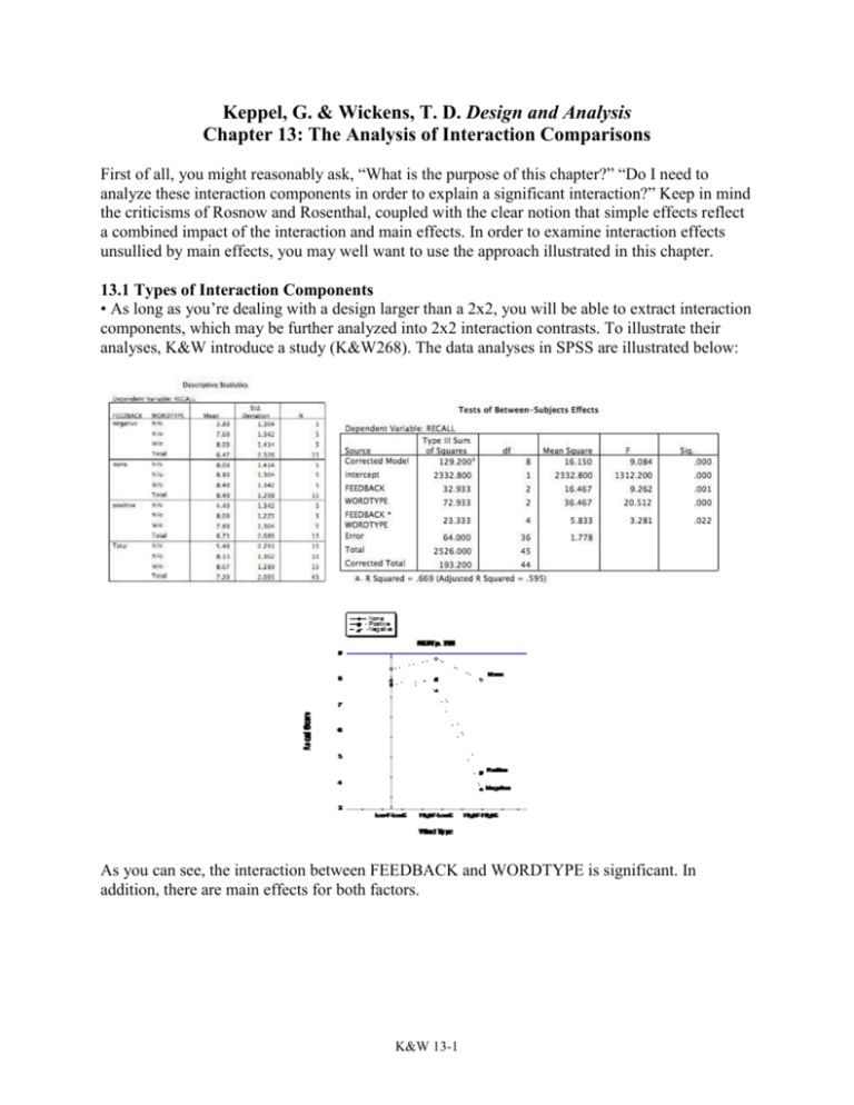
analyses, K&W introduce a study (K&W268). The data analyses in SPSS are illustrated below:
As you can see, the interaction between FEEDBACK and WORDTYPE is significant. In
addition, there are main effects for both factors.
K&W 13-1
• Because we need to know if we have a problem with heterogeneity of variance, I’ll conduct the
Brown-Forsythe test:
There appears to be no reason to be concerned about heterogeneity of variance.
Interaction of a Contrast and a Factor
• In order to interpret the interaction, you could look at the simple effects (as discussed in Ch.
12). That is, you could look at the effects of WORDTYPE at each level of FEEDBACK
separately. Alternatively, you could look at the effects of WORDTYPE at more than one level of
FEEDBACK simultaneously. In so doing, you could determine if there appears to be an
interaction between the two factors, but only for particular levels of one factor.
• To my eyes, it appears that providing no feedback has little impact on recall performance,
regardless of the type of word (recall is fairly high for all types of word when no feedback is
given). Moreover, it appears that positive and negative feedback both have a similar impact on
recall. Thus, for both of these types of feedback, recall seems to be higher for low emotion words
than for high emotion words. Thus, I might look at the simple effect of WORDTYPE for each
level of FEEDBACK.
• As K&W indicate, in an effort to understand the 3x3 interaction, you could look at three
separate 2x3 interaction components, as seen below:
Pos
Neg
lolo
7.8
8.0
F=
hilo
8.0
7.6
.433
= .243
1.778
hihi
4.4
3.8
None
Pos
lolo
8.4
7.8
F=
hilo
8.8
8.0
7.033
= 3.96
1.778
hihi
8.0
4.4
None
Neg
lolo
8.4
8.0
F=
hilo
8.8
7.6
hihi
8.0
3.8
10.033
= 5.64
1.778
• Just so it’s clear, for WORDTYPE, hihi = high-frequency words with high emotional content,
hilo = high-frequency words with low emotional content, and lolo = low-frequency words with
low emotional content.
K&W 13-2
• The three ANOVAs printed above are not particularly helpful, because all that you’re really
interested in determining is whether or not an interaction is present. To that end, you want to
assess the interaction term, but the MSError you want is from the overall ANOVA, given
homogeneity of variance. For the moment, let’s not worry about whether or not the interaction is
significant or not, because that would require that we determine if we would consider the
assessment as a post hoc test or not. The obtained F-ratios for the three interactions are seen
below the source tables above.
• Because there appears to be little difference in the impact of positive and negative feedback,
illustrated above with a very small F for the interaction between positive and negative feedback,
it would make sense to lump together those two types of feedback. To do so, I would construct a
“complex” interaction, in which two levels of a factor are averaged. In this case, it’s possible to
compare the No Feedback group (None) to a Feedback group (average of Pos and Neg
feedback).
None
Feedback
lolo
8.4
7.9
hilo
8.8
7.8
hihi
8.0
4.1
F=
11.233
= 6.32
1.778
• The consolidation of two levels of a factor into a single level often makes sense, simplifying
the writing of the results. Although K&W don’t provide any analyses at this point, you should
see that the apparent interaction of type of word with feedback vs. no feedback could now be
investigated to provide an assessment of the results of this study.
• As K&W observe, it’s also possible to look at the interactions of WORDTYPE crossed with
FEEDBACK. Then, one might combine the two types of contrasts.
Interaction of Two Contrasts: Interaction Contrasts
• “Many of the most useful interaction contrasts are formed by crossing two pairwise contrasts.
The resulting interaction contrast extracts a 2x2 subtable of the original means.”
• “Researchers trying to understand this type of interaction often reduce a large table to a series
of pairwise subtables and examine the interaction within each. This strategy is, for interactions,
much like looking at the set of pairwise comparisons for main effects.”
• K&W illustrate a number of 2x2 interaction contrasts that one could construct for this data set.
For example, you could compare high and low frequency words with low emotion at each pair of
feedback possibilities:
Pos
Neg
F=
lolo
7.8
8.0
hilo
8.0
7.6
.450
= .253
1.778
lolo
8.4
7.8
None
Pos
F=
hilo
8.8
8.0
.05
= .03
1.778
K&W 13-3
None
Neg
F=
lolo
8.4
8.0
hilo
8.8
7.6
.80
= .45
1.778
hilo
8.0
7.6
Pos
Neg
F=
hihi
4.4
3.8
.05
= .03
1.778
hilo
8.8
8.0
None
Pos
F=
hihi
8.0
4.4
9.8
= 5.51
1.778
hilo
8.8
7.6
None
Neg
F=
hihi
8.0
3.8
11.25
= 6.33
1.778
13.2 Analyzing Interaction Contrasts
• K&W provide the necessary formulas for computing the interaction contrasts. These formulas
will serve you well when stranded on a desert island.  What you need to recognize is that these
interaction contrasts are essentially the interaction components of an ANOVA, as I’ve illustrated
above. Thus, to use SPSS to compute the first numerical example on p. 274, you would need to
Select Cases so that you’re left with only the Positive and Negative feedback conditions and only
the hilo and hihi word types. That’s the interaction depicted above on the far left (F = .03).
• Had you first collapsed the two feedback groups into a single group (as illustrated a bit earlier,
with the resulting 2x3 analysis), you might then construct individual 2x2 analyses to determine
the source of the resulting interaction. K&W illustrate one such 2x2 on p. 274, for no feedback
vs. feedback (A4 = 2, -1, -1) and high frequency words with low vs. high emotion (B2 = 0, 1, -1).
To compute this “complex” comparison in SPSS, you’d need to change your Positive and
Negative feedback values to a single value (e.g., Feedback) so that your FEEDBACK variable
takes on only two values (None and Feedback). Then, you would need to select cases to
eliminate the lolo WORDTYPE. That analysis is seen below on the far right.
None
Feedback
F=
lolo
8.4
7.9
hilo
8.8
7.8
.417
= .23
1.778
None
Feedback
F=
lolo
8.4
7.9
hihi
8.0
4.1
11.233
= 6.32
1.778
None
Feedback
F=
hilo
8.8
7.8
hihi
8.0
4.1
14.017
= 7.88
1.778
• As noted earlier, given the non-significant Brown-Forsythe test above, we would use the
MSError from the overall ANOVA (1.778) to construct the F-ratios for any interaction contrasts.
In the absence of homogeneity of variance, you would use an error term that comes from the
conditions involved in the specific contrast (i.e., you would use the F-ratio that appears in the
source tables above).
• Of course, although K&W don’t really provide an interpretation, what you really want to know
is how to interpret the interaction. Given the pattern of interaction contrasts, here’s what I would
propose. The effect of positive and negative feedback was similar, so I would collapse those two
K&W 13-4
levels and compare feedback (of any sort) with no feedback. Then it appears that the impact of
type of feedback (none vs. some) on recall is similar when dealing with low emotion words
(whether low or high frequency), resulting in no 2x2 interaction, F = .23. Next, it appears that
recall of low emotion words differs from high emotion words as a function of feedback,
primarily due to the low recall of high emotion words. However, to fully appreciate what’s going
on, I would feel more comfortable using a post hoc statistical analysis. Using the Fisher-Hayter
approach, I would get the following critical mean difference:
DFH = qa-1
MSError
1.778
= 4.07
= 2.43
n
5
Doing so would lead me to the following interpretation…
There was a significant interaction between types of feedback and types of word, F(4,36) =
3.281, MSE = 1.778, p = .022. Subsequent analyses of interaction components indicated that the
impact of positive and negative feedback was equivalent, so these two levels were combined into
a single level. Thus, the interaction was collapsed into a 2 (No Feedback vs. Feedback) x 3 (Low
Frequency/Low Emotion Words, High Frequency/Low Emotion Words, and High
Frequency/High Emotion Words) interaction. A series of 2x2 interaction contrasts, coupled with
a Fisher-Hayter analysis, indicated a different pattern for low emotion and high emotion words.
As seen in Figure 1 (below), low emotion words, regardless of frequency, were recalled quite
well regardless of type of feedback. Mean recall for these four conditions ranged between 7.8
and 8.8, with none of the means differing significantly. When low emotion words were
compared to high emotion words, however, feedback did have an impact. When there was no
feedback, the low emotion words (whether low or high in frequency) and high emotion words
were recalled equally well (with means ranging from 8.0 to 8.8). However, when feedback was
given, low emotion words (whether low, M = 7.9, or high in frequency, M = 7.8) were recalled
better than high emotion words (M = 4.1), which were also high in frequency. [To be honest, I’d
be more comfortable with this study if it included low frequency words that were high in
emotion!]
K&W 13-5
13.3 Orthogonal Interaction Contrasts
• Interaction contrasts are the smallest units of analysis for an interaction. Unlike simple effects,
which reflect both interaction and main effects, interaction contrasts “are orthogonal to both of
the main effects and any main comparisons.”
• A set of orthogonal interaction contrasts will fully exhaust the SSInteraction. For any interaction,
there will be (a – 1)(b – 1) orthogonal interaction contrasts.
• K&W show a set of orthogonal interaction contrasts for a 3x3 design in Table 13.5.
B1
B2
1
-½
-½
0
1
-1
A1
-1
-1
½
½
-1
0
-1
1
0
0
0
0
0
0
0
0
1
1
-½
-½
1
0
1
-1
1
-½
-½
0
1
-1
A2
-1
-1
½
½
-1
0
-1
1
2
2
-1
-1
2
0
2
-2
-1
-1
½
½
-1
0
-1
1
You can demonstrate orthogonality by the usual process of multiplication and then summing the
products to ensure that the result is 0. For example, to compare the coefficients for A1xB1 with
those for A2xB1, you would multiply all the coefficients in the same “location” and then sum:
(-1 x -1) + (.5 x .5) + (.5 x .5) + (0 x 2) + (0 x -1) + (0 x -1) + (1 x -1) + (-.5 x .5) + (-.5 x .5) = 0.
• As was true for the earlier discussion of orthogonal contrasts, you wouldn’t compute
orthogonal interaction contrasts if they were not of theoretical interest.
13.4 Testing Contrast-by-Factor Interactions
• Because they will not necessarily be 2x2 contrasts, the contrast-by-factor interactions are less
specific than interaction contrasts. To illustrate the process, K&W describe a study about
electrical self-stimulation of the brain by rats. Though they don’t provide the raw data, I’ve
constructed a data set that is roughly equivalent to the one producing the means in Table 13.6.
The SPSS output would look like this:
K&W 13-6
• Note, first of all, that all effects are significant. However, because the interaction is significant,
that’s where we would focus our attention. As you look at the graph, it should occur to you that
for Brain Areas 1 and 3 there is little change in the number of shocks administered as a function
of intensity. Thus, you might even consider the possibility of collapsing these two levels into a
single area, as was done for the earlier example. Note, however, that for Brain Area 2, number of
shocks appears to be greater when administered with Intensities 3, 4, and 5 compared to Intensity
1 and maybe even Intensity 2.
• K&W provide two formulas for the contrast-by-factor interaction:
SSy A xB =
(
n å k yˆ A.at.bk - yˆ A
åc
2
j
SSy A xB = å SSy A .at.bk - SSy A
)
2
(13.10)
(13.11)
The first formula is direct, while the second relies on the fact that the sum of the SS for simple
effects is equal to the SSMain Effect plus the SSInteraction (with some substitution and rearrangement of
terms).
• K&W approach this analysis using linear {-2, -1, 0, 1, 2} and quadratic {2, -1, -2, -1, 2}
contrasts. To compute the  values, you can use the formulas that K&W provide. It’s fairly easy,
however, to generate the  values in SPSS. First, you need to select cases sequentially so that
Brain Area equals 1, then 2, then 3. At each Brain Area, you could use Compare Means->OneWay ANOVA to compute the appropriate contrast. After entering the two contrasts, I’d get the
following output for each of the three brain areas:
Brain Area b1
Brain Area b2
K&W 13-7
Brain Area b3
Using the overall means (rather than means at each specific brain area), the linear and quadratic
contrasts would yield the following information:
Of course, the t-statistics computed by SPSS aren’t useful as printed, because they are based on
the wrong error term. (Note that the analysis is a one-way ANOVA, which would use an error
term that mixes in the effects of intensity.) However, the Value of Contrast as printed is an
estimate of  for each contrast. That is helpful! Thus, SPSS will generate the estimated  terms,
which are the same as K&W show in Table 13.7 (and seen below, which are the same except for
some rounding differences).
Linear
yˆ
b1
b2
b3
YA j
-0.2
12.8
-1.2
3.8
SS
0.02
81.92
0.72
21.66
yˆ
Quadratic
SS
0.01
51.43
0.70
20.74
0.2
-12.0
-1.4
-4.4
• We can now use Equation 13.10 to compute the SS for the linear interaction component.
SSy A xB =
(
n å k yˆ A.at.bk - yˆ A
åc
2
j
)
2
(5)[(-0.2 - 3.798) 2 + (12.8 - 3.798) 2 + (-1.2 - 3.798) 2 ]
=
= 61.0
(-2) 2 + (-1) 2 + (0) 2 + (1) 2 + (2) 2
• Alternatively, you could use Equation 13.11 to compute SS for the linear interaction
component.
SSy A xB = å SSy A .at.bk - SSy A = (0.02 + 81.92 + 0.72) - 21.64 = 61.0
• To compute the MS for this contrast, you need df.
dfy A xB = dfy A ´ df B = (1)(b -1) = b -1
K&W 13-8
(13.12)
So, in this case MSA linear xB =
61.0
= 30.5 and F = 30.5 / 3.31 = 9.21.
2
After establishing that this result is significant, one would need to compute subsequent analyses
on the simple linear contrasts (with the linear trend at b2 significant and not significant at b1 and
b3). K&W also talk about analyzing the quadratic component or all non-linear components.
• As I noted earlier, however, it appears that b1and b3 are not much different. I could establish
that they are similar by comparing them in a 2x5 analysis. If there are no main effects or
interactions, I would feel comfortable combining those two levels and then re-analyzing the
results as a 2 (b2 vs. b1+b3) x 5 (Intensity) analysis. The ANOVA suggests that those two levels
really don’t differ that much.
Thus, I would combine those two levels into a single level (found in a new variable called
combo) and re-compute the ANOVA:
As you can see, the main effects of area and intensity are still significant, as is the interaction.
• First, let me compute a simple effects analysis of intensity at the combined brain area (area1 +
area3).
K&W 13-9
As you know, the F is not accurate, because I need to divide the MSEffect by the MSError from the
overall ANOVA (with the combined data). Thus F = .808 / 3.15 = .26. Clearly, the combined
brain areas are little affected by the intensity.
• Next, let me compute a simple effects analysis of intensity at brain area 2.
Again, you’d need to compute the appropriate F using the MSError from the overall ANOVA: F =
33.54 / 3.15 = 10.65. Clearly that’s a big effect.
• Thus, it appears that the interaction emerges because intensity has an impact on performance in
Brain Area 2, but not in Brain Areas 1 or 3. What is that effect? I could compare the five means
using a critical mean difference (e.g., Fisher-Hayter). Because the interaction we’re trying to
explain now comes from 10 means, I obtained q using 9 means and dfError = 65. Then, because
five of the means had sample size n = 5 and half had sample size n = 10, I took the mean for the
denominator under the radical.
3.15
DF- H = 4.55
= 2.95
7.5
• For Brain Area 2, there appears to be an intensity that is not effective (1), because the rats selfstimulate at the lowest level (M = 1.3) compared to all the other intensity levels. Although two
levels (3 and 4) seem optimal, because the rats self-stimulate at the highest levels (M = 7.3 and M
= 7.7, respectively), those values are not significantly greater than levels of self-stimulation for
intensities 2 and 5 (M = 4.7 and M = 6.2, respectively). However, for Brain Areas 1 and 3, rates
of self-stimulation were low (overall M = 2.47) and did not differ regardless of intensity. Clearly,
stimulating these two brain areas is not rewarding for the rats, because they don’t choose to
stimulate themselves often, regardless of intensity.
13.5 Contrasts Outside the Factorial Structure
• Given one’s theoretical interests, there may be unusual contrasts that make sense. K&W show
how you can compute these contrasts. However, I’d bet that you’d only rarely be inclined to do
so. When you are so inclined, you may come back and review this portion of the chapter. 
13.6 Multiple Tests and Type I Error
• As always, if your contrasts are planned (and you aren’t afraid of a skeptical journal editor),
you could conduct a reasonable number of those tests without a correction for familywise Type I
error. On the other hand, you may invoke some form of correction and the Sidák-Bonferroni
procedure makes sense, possibly with FW = .10.
K&W 13-10