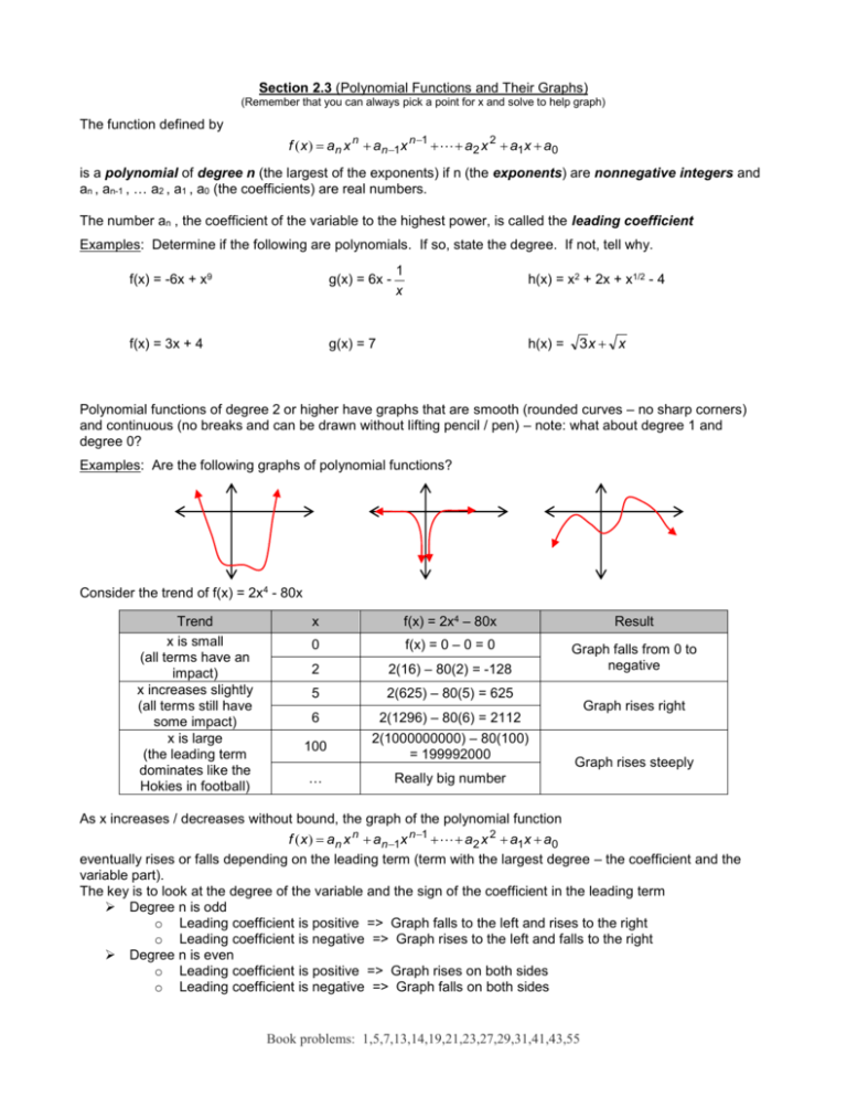
Section 2.3 (Polynomial Functions and Their Graphs)
(Remember that you can always pick a point for x and solve to help graph)
The function defined by
f ( x )  an x n  an 1x n 1    a2 x 2  a1x  a0
is a polynomial of degree n (the largest of the exponents) if n (the exponents) are nonnegative integers and
an , an-1 , … a2 , a1 , a0 (the coefficients) are real numbers.
The number an , the coefficient of the variable to the highest power, is called the leading coefficient
Examples: Determine if the following are polynomials. If so, state the degree. If not, tell why.
f(x) = -6x + x9
g(x) = 6x -
f(x) = 3x + 4
g(x) = 7
1
x
h(x) = x2 + 2x + x1/2 - 4
h(x) =
3x  x
Polynomial functions of degree 2 or higher have graphs that are smooth (rounded curves – no sharp corners)
and continuous (no breaks and can be drawn without lifting pencil / pen) – note: what about degree 1 and
degree 0?
Examples: Are the following graphs of polynomial functions?
Consider the trend of f(x) = 2x4 - 80x
Trend
x is small
(all terms have an
impact)
x increases slightly
(all terms still have
some impact)
x is large
(the leading term
dominates like the
Hokies in football)
x
f(x) = 2x4 – 80x
0
f(x) = 0 – 0 = 0
2
2(16) – 80(2) = -128
5
2(625) – 80(5) = 625
6
2(1296) – 80(6) = 2112
100
2(1000000000) – 80(100)
= 199992000
…
Really big number
Result
Graph falls from 0 to
negative
Graph rises right
Graph rises steeply
As x increases / decreases without bound, the graph of the polynomial function
f ( x )  an x n  an 1x n 1    a2 x 2  a1x  a0
eventually rises or falls depending on the leading term (term with the largest degree – the coefficient and the
variable part).
The key is to look at the degree of the variable and the sign of the coefficient in the leading term
 Degree n is odd
o Leading coefficient is positive => Graph falls to the left and rises to the right
o Leading coefficient is negative => Graph rises to the left and falls to the right
 Degree n is even
o Leading coefficient is positive => Graph rises on both sides
o Leading coefficient is negative => Graph falls on both sides
Book problems: 1,5,7,13,14,19,21,23,27,29,31,41,43,55
Examples: Look at the chart on page 304 and use the Leading Coefficient Test to determine the end behavior
of the graph of the following
f(x) = 3x7 – 2x5 – 4x2 + 6
g(x) = 8x6 + 4x5 + 8
h(x) = -4x4 + 3
The values of x for which the polynomial function f(x) is equal to 0 are called the zeros of f (also called the roots
or solutions of f). Each real root is an x-intercept of the graph of the polynomial function.
Example: Find all zeros of…
f(x) = x3 + 2x2 – 4x – 8
g(x) = x4 – 4x2
In the 2nd example just shown, the factorization was g(x) = x2(x + 2)(x – 2). The factor x occurs twice and the
factors (x + 2) and (x – 2) occur once. The number of times a factor occurs gives the multiplicity of that zero.
So our solution 0 has multiplicity 2 and our solutions 2 and -2 have multiplicity 1.
If a zero (solution) has even multiplicity, the graph touches the x-axis at this point and turns around. If a zero
(solution) has odd multiplicity, the graph crosses the x-axis at this point.
Example: Find the zeros / the multiplicity of each zero, and state the behavior of the graph at each zero
g(x) = x4 – 4x2
f(x) = -4(x + ½)2(x – 5)3
You can use the facts learned in this section and other steps mentioned (pg. 310) to sketch graphs of
polynomial functions (note additional steps of finding y-intercept by finding f(0) and determining possible
symmetry by looking at f(-x) = f(x) : y-axis symmetry, f(-x) = -f(x) : origin symmetry)
Examples: After reviewing the chart and steps on pg. 310, use those steps to graph x 3 – 3x2 on the board
Book problems: 1,5,7,13,14,19,21,23,27,29,31,41,43,55