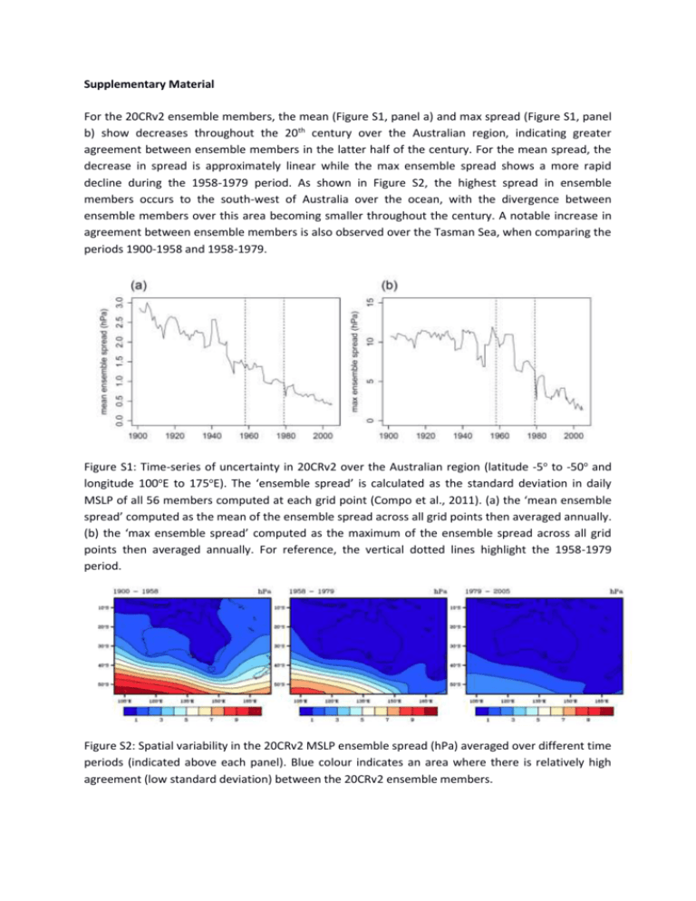
Supplementary Material
For the 20CRv2 ensemble members, the mean (Figure S1, panel a) and max spread (Figure S1, panel
b) show decreases throughout the 20th century over the Australian region, indicating greater
agreement between ensemble members in the latter half of the century. For the mean spread, the
decrease in spread is approximately linear while the max ensemble spread shows a more rapid
decline during the 1958-1979 period. As shown in Figure S2, the highest spread in ensemble
members occurs to the south-west of Australia over the ocean, with the divergence between
ensemble members over this area becoming smaller throughout the century. A notable increase in
agreement between ensemble members is also observed over the Tasman Sea, when comparing the
periods 1900-1958 and 1958-1979.
Figure S1: Time-series of uncertainty in 20CRv2 over the Australian region (latitude -5o to -50o and
longitude 100oE to 175oE). The ‘ensemble spread’ is calculated as the standard deviation in daily
MSLP of all 56 members computed at each grid point (Compo et al., 2011). (a) the ‘mean ensemble
spread’ computed as the mean of the ensemble spread across all grid points then averaged annually.
(b) the ‘max ensemble spread’ computed as the maximum of the ensemble spread across all grid
points then averaged annually. For reference, the vertical dotted lines highlight the 1958-1979
period.
Figure S2: Spatial variability in the 20CRv2 MSLP ensemble spread (hPa) averaged over different time
periods (indicated above each panel). Blue colour indicates an area where there is relatively high
agreement (low standard deviation) between the 20CRv2 ensemble members.
Figure S3: Violin plots displaying distribution of Pearson pattern correlations under different
node configurations in the ‘historical’ SOM (as related to the SOM presented in Figure 1 of
main manuscript). For each node configuration, a standard box-plot is shown inside a kernel
density plot. (a) Pattern correlations between the SOM node to which the daily MSLP field was
classified into and the actual MSLP field. This distribution of pattern correlations is a measure of
the ‘realism’ of the node pattern. (b) Pattern correlations between each possible SOM node
pair for the particular node configuration. This distribution of pattern correlations is a
measure of the differences between nodes, which desirably has a large enough range and
low enough median so that the nodes sample a range of the different circulation patterns
present in the MSLP field.