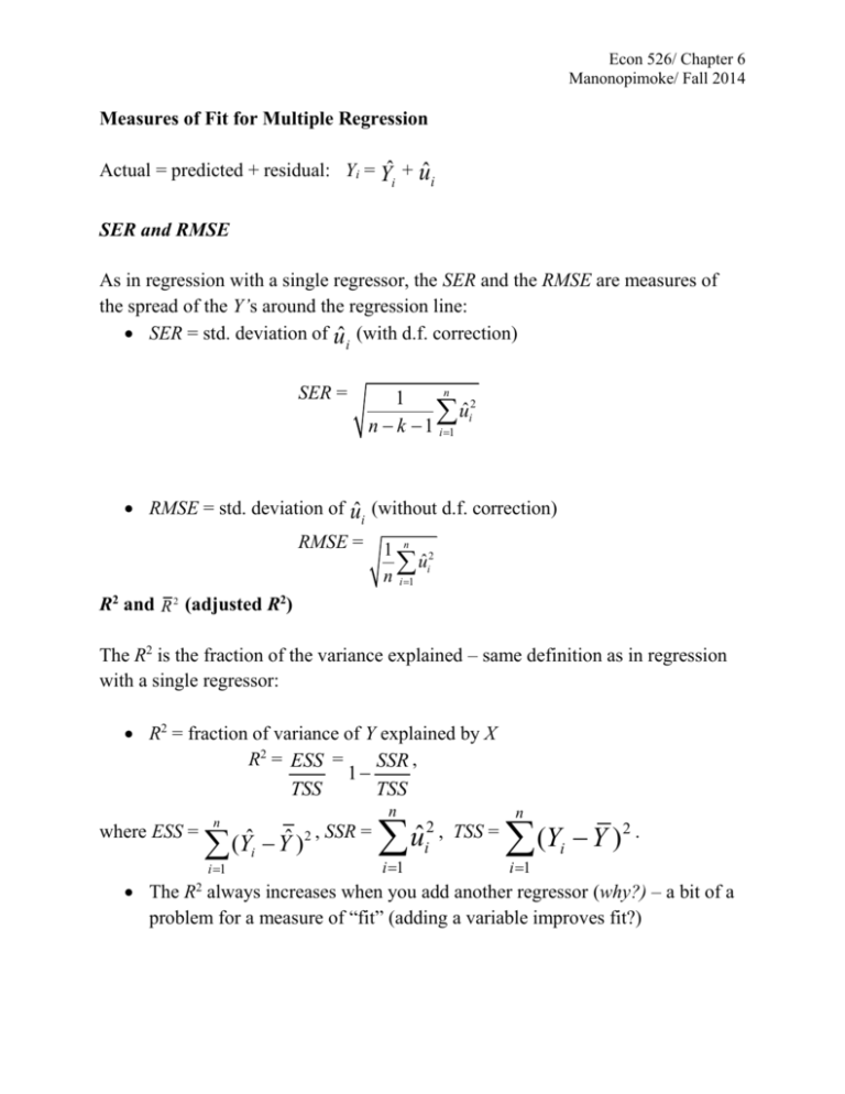
Econ 526/ Chapter 6
Manonopimoke/ Fall 2014
Measures of Fit for Multiple Regression
Actual = predicted + residual: Yi = Yˆ + uˆ
i
i
SER and RMSE
As in regression with a single regressor, the SER and the RMSE are measures of
the spread of the Y’s around the regression line:
 SER = std. deviation of uˆ (with d.f. correction)
i
SER =
n
1
uˆi2

n  k  1 i 1
 RMSE = std. deviation of uˆ (without d.f. correction)
i
RMSE =
1 n 2
 uˆi
n i 1
R2 and R 2 (adjusted R2)
The R2 is the fraction of the variance explained – same definition as in regression
with a single regressor:
 R2 = fraction of variance of Y explained by X
R2 = ESS =
SSR ,
1
TSS
TSS
where ESS =
n
 (Yˆi  Yˆ )
i 1
n
2 , SSR =
 uˆ
i 1
2 , TSS =
i
n
 (Y  Y )
i 1
2.
i
 The R always increases when you add another regressor (why?) – a bit of a
problem for a measure of “fit” (adding a variable improves fit?)
2
Econ 526/ Chapter 6
Manonopimoke/ Fall 2014
The R 2 (the “adjusted R2”) corrects this problem by “penalizing” you for including
another regressor – the R 2 does not necessarily increase when you add another
regressor.
R 2 = “adjusted R2” = R2 with a degrees-of-freedom correction that adjusts for
estimation uncertainty; R 2 < R2 as the correction is always larger than 1 however if
n is large the two will be very close
Adjusted R2: R 2 =
 n  1  SSR
1 

 n  k  1  TSS
Test score example:
(1)
= 698.9 – 2.28STR,
̂
𝑇𝑒𝑠𝑡𝑠𝑐𝑜𝑟𝑒
R2 = .05, SER = 18.6
(2)
̂ = 686.0 – 1.10STR – 0.65PctEL,
𝑇𝑒𝑠𝑡𝑠𝑐𝑜𝑟𝑒
R2 = .426, R 2 = .424, SER = 14.5
 What – precisely – does this tell you about the fit of regression (2) compared
with regression (1)?
 Why are the R2 and the R 2 so close in (2)?
Econ 526/ Chapter 6
Manonopimoke/ Fall 2014
The Least Squares Assumptions for Multiple Regression
Yi = 0 + 1X1i + 2X2i + … + kXki + ui, i = 1,…,n
Assumption #1: the conditional mean of u given the included Xs is zero.
E(u|X1 = x1,…, Xk = xk) = 0
 This has the same interpretation as in regression with a single regressor.
 Failure of this condition leads to omitted variable bias, specifically, if an
omitted variable
(1) belongs in the equation (so is in u) and
(2) is correlated with an included X
 The best solution, if possible, is to include the omitted variable in the
regression. A second, related solution is to include a variable that
controls for the omitted variable (discussed in Ch. 7)
Assumption #2: (X1i,…,Xki,Yi), i =1,…,n, are i.i.d.
This is satisfied automatically if the data are collected by simple random
sampling.
Assumption #3: E( X 4 ) < ∞,…, E( X 4 ) < ∞, and E(Y 4 ) < ∞. Large outliers
i
1i
ki
are rare (finite fourth moments). Plot your data!
This is the same assumptions as we had before for a single regressor.
Econ 526/ Chapter 6
Manonopimoke/ Fall 2014
Assumption #4: There is no perfect multicollinearity
Perfect multicollinearity is when one of the regressors is an exact linear function
of the other regressors.
Example: Suppose you accidentally include STR twice:
regress testscr str str, robust
Regression with robust standard errors
Number of obs = 420
F( 1, 418) = 19.26
Prob > F = 0.0000
R-squared = 0.0512
Root MSE = 18.581
------------------------------------------------------------------------|
Robust
testscr | Coef. Std. Err. t P>|t| [95% Conf. Interval]
--------+---------------------------------------------------------------str | -2.279808 .5194892 -4.39 0.000 -3.300945 -1.258671
str | (dropped)
_cons | 698.933 10.36436 67.44 0.000 678.5602 719.3057
------------------------------------------------------------------------ In the previous regression, 1 is the effect on TestScore of a unit change in STR,
holding STR constant (???)  STATA drops STR or will refuse to calculate the
OLS estimates and give an error message.
 We will return to perfect (and imperfect) multicollinearity shortly, with more
examples…
Econ 526/ Chapter 6
Manonopimoke/ Fall 2014
The Sampling Distribution of the OLS Estimator
Under the four Least Squares Assumptions,
 The sampling distribution of ˆ has mean 1
1
 var( ˆ ) is inversely proportional to n.
1
 Other than its mean and variance, the exact (finite-n) distribution of ˆ is
1
very complicated; but for large n…
p
o ˆ is consistent: ˆ  1 (law of large numbers)
1
1
o ˆ
is approximately distributed N(0,1) (CLT)
1  E ( ˆ1 )
var( ˆ )
1
o These statements hold for ˆ ,…, ˆ
1
k
Multicollinearity, Perfect and Imperfect
Perfect multicollinearity is when one of the regressors is an exact linear function
of the other regressors.
Some more examples of perfect multicollinearity
1.
The example from before: you include STR twice,
2.
Regress TestScore on a constant, D, and B, where: Di = 1 if STR ≤ 20,
= 0 otherwise; Bi = 1 if STR >20, = 0 otherwise, so Bi = 1 – Di and
there is perfect multicollinearity. (i.e. B_i can be written as a perfect
linear combination of D_i)
The dummy variable trap
Suppose you have a set of multiple binary (dummy) variables, which are
mutually exclusive and exhaustive – that is, there are multiple categories and every
observation falls in one and only one category (5 race groups: African American,
Asian, Hispanic, All others). If you include all these dummy variables and a
constant, you will have perfect multicollinearity.
Econ 526/ Chapter 6
Manonopimoke/ Fall 2014
 Why is there perfect multicollinearity here?
Let B i, Ai, Hi,Ni, Oi be dummy variables for black, Asian, Hispanic, and native
americans and others respectfully.
The usual way to avoid this is to exclude one of the binary variables. Let’s say we
exclude the Oi group:
The coefficients on the included binary variables represent the incremental effect
of being in that category relative to the base case of the omitted category holding
constant other regressors.
Alternatively, we can exclude the intercept.
Econ 526/ Chapter 6
Manonopimoke/ Fall 2014
 Perfect multicollinearity usually reflects a mistake in the definitions of the
regressors, or an oddity in the data
 If you have perfect multicollinearity, your statistical software will let you know
– either by crashing or giving an error message or by “dropping” one of the
variables arbitrarily
 The solution to perfect multicollinearity is to modify your list of regressors so
that you no longer have perfect multicollinearity.
Imperfect multicollinearity occurs when two or more regressors are very highly
correlated. In this case, one or more of the regression coefficients will be
imprecisely estimated.
e.g. including percentage of the districts’ residents who are first generation
immigrants and percentage of English learners (PctEL) both as regressors. It would
be difficult to use these data to estimate the partial effect on test scores of an
increase in PctEL holding constant the percentage immirgrants
The idea: the coefficient on X1 is the effect of X1 holding X2 constant; but if X1 and
X2 are highly correlated, there is very little variation in X1 once X2 is held constant
– so the data don’t contain much information about what happens when X1 changes
but X2 doesn’t. If so, the variance of the OLS estimator of the coefficient on X1
will be large.
 Imperfect multicollinearity (correctly) results in large standard errors for one
or more of the OLS coefficients. OLS estimates will be unbiased.
 The math? See SW, App. 6.2
Next topic: hypothesis tests and confidence intervals…