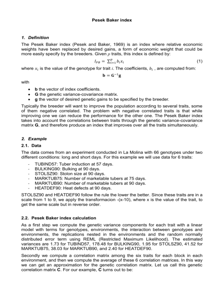
Pesek Baker index
1. Definition
The Pesek Baker index (Pesek and Baker, 1969) is an index where relative economic
weights have been replaced by desired gains, a form of economic weight that could be
more easily specify by the breeders. Given p traits, this index is defined by:
𝐼𝑃𝐵 = ∑𝑝𝑖=1 𝑏𝑖 𝑥𝑖
(1)
where 𝑥𝑖 is the value of the genotype for trait i. The coefficients, 𝑏𝑖 , are computed from:
𝐛 = 𝐆−1 𝐠
with



b the vector of index coefficients.
G the genetic variance-covariance matrix.
g the vector of desired genetic gains to be specified by the breeder.
Typically the breeder will want to improve the population according to several traits, some
of them negative correlated. The problem with negative correlated traits is that while
improving one we can reduce the performance for the other one. The Pesek Baker index
takes into account the correlations between traits through the genetic variance-covariance
matrix G, and therefore produce an index that improves over all the traits simultaneously.
2. Example
2.1. Data
The data comes from an experiment conducted in La Molina with 66 genotypes under two
different conditions: long and short days. For this example we will use data for 6 traits:
-
TUBIND57: Tuber induction at 57 days.
BULKING90: Bulking at 90 days.
STOLSZ90: Stolon size at 90 days.
MARKTUB75: Number of marketable tubers at 75 days.
MARKTUB90: Number of marketable tubers at 90 days.
HEATDEF90: Heat defects at 90 days.
STOLSZ90 and HEATDEF90 follow the rule the lower the better. Since these traits are in a
scale from 1 to 9, we apply the transformacion -(x-10), where x is the value of the trait, to
get the same scale but in reverse order.
2.2. Pesek Baker index calculation
As a first step we compute the genetic variance components for each trait with a linear
model with terms for genotypes, environments, the interaction between genotypes and
environments, the replications nested in the environments and the random normally
distributed error term using REML (Restricted Maximum Likelihood). The estimated
variances are 1.73 for TUBIND57, 178.48 for BULKING90, 1.95 for STOLSZ90, 41.52 for
MARKTUB75, 38.03 for MARKTUB90, and 2.40 for HEATDEF90.
Secondly we compute a correlation matrix among the six traits for each block in each
environment, and then we compute the average of these 6 correlation matrices. In this way
we can get an approximation for the genetic correlation matrix. Let us call this genetic
correlation matrix C. For our example, C turns out to be:
1 0.0657 0.3787 0.1582 0.0301 0.3240 

1
0.1781 0.4422 0.6802 0.1373 


1
0.1698  0.0805 0.4221 
C
.
1
0.4373 0.0830 


1
 0.0004


1


Multiplying the entries of this genetic correlation matrix with the corresponding variances
and standard deviations computed in the first step, we can get an approximation for the
genetic variance-covariance matrix G. The resulting matrix for our data is:
0.6609 
1.735 1.157 0.6966 1.343 0.2441

178.5 3.324 38.07 56.04
2.841 


1.951 1.529  0.6932
0.9130 
G
.
41.52 17.38
0.8281 


38.03  0.003540


2.398 

We can also compute heritabilities with the variance components estimated in the first step
using formula
h2 
 
2
G
 G2
 G2 E
e

 e2
(2)
er
2
where 𝜎𝐺2 is the genetic variance, 𝜎𝐺×𝐸
is the variance for the interaction between
2
genotypes and environments, 𝜎𝑒 is the error variance, e the number of environments (2 in
this case) and r the number of replications (3 in this case). Here we get:
78.88
78.25




81
.
89
h2  
.
64
.
90


57.29


84.47 
Now we need to define the vector of desired genetic gains, g. A good practice in order to
get a sensible index that accommodates all the traits and gives an appropriate weight to all
of them is to use the standard deviations for g, so we have:
1.317 
13.36 


1.397 
g
.
6.444
6.166


1.548 
Finally, the index coefficients are:
0.3934
0.0046




0
.
3986
b  G 1g  
.
0.0610
0.1322


0.3592
(3)
Heritability is defined by the ratio between the genetic and the phenotypic variance. From
formula (2) we see that the phenotypic variance for this example is defined by
 P2   G2 
 G2 E

 e2
.
e
er
We have estimates for the phenotypic variances that have been used to compute the
heritabilities. Using these estimates and the covariances on matrix G, we can estimate a
phenotypic covariance matrix P:
0.6609 
2.199 1.157 0.6966 1.343 0.2441

228.1 3.324 38.07 56.04
2.841 


2.383 1.529  0.6932
0.9130 
P
.
63
.
97
17
.
38
0
.
8281



66.38  0.003540


2.839 

Now we can compute the response to selection for each trait using formula
Rj  i
b'c j
b' Pb V ( y j )
where i is the selection intensity that corresponds to a selected fraction , cj is the j-th
column of matrix G and V(yj) the variance for trait j.
For our example, if we want to select the superior 10%, then the 0.9 quantil of the normal
distribution is 1.282, the ordinate of the normal density at this point is 0.1755 and the
selection intensity is
i
0.1755
 1.755 .
0.1
The b' Pb product is 3.679, and the response to selection for each trait result (below the
example for trait 1):
R1  1.755 
0.39  1.73  0.0046  1.16  0.40  0.70  0.061  1.34  0.13  0.24  0.36  0.66
3.679  1.73
 0.915
Since we are using standardized units (remember we used the standard deviations in
vector g to compute b, see formula (3)), we will get the same result for each trait, so the
response to selection is 0.915 standard deviations. We can multiply this value by the
standard deviations to get the response to selection in actual units:

For TUBIND57: 0.915 × 1.3171 = 1.205 points.

For BULKING90: 0.915 × 13.3595 = 12.22 %.

For STOLSZ90: 0.915 × 1.3969 = 1.278 points.

For MARKTUB75: 0.915 × 6.4437 = 5.895 tubers.

For MARKTUB90: 0.915 × 6.1665 = 5.642 tubers.

For HEATDEF90: 0.915 × 1.5485 = 1.417 points.
An important question is how this selection index correlates with each of the traits. To see
this we plot the index and the mean value of the trait for each genotype.
Let us see now how the index behaves for each environment. For the short days
environment we have
and for the long days environment
Which are the best clones according to this index? In the table below we show the top 10
clones over both environments and in each environment.
Top 10 clones selected with the Pesek Baker index in two environments
Ranking
Best over both
environments
Best on the short days
environment
Best on the long days
environment
1
CIP-300072.1
CIP-300072.1
CIP-300072.1
2
CIP-300048.12
CIP-301023.15
CIP-300048.12
3
Atlantic
CIP-300056.33
Atlantic
4
CIP-397077.16
CIP-300048.12
CIP-390478.9
5
CIP-390478.9
CIP-397077.16
CIP-397077.16
6
CIP-301023.15
CIP-301024.14
CIP-300054.29
7
CIP-392973.48
CIP-392973.48
CIP-392973.48
8
CIP-300056.33
CIP-390478.9
CIP-397014.2
9
CIP-388676.1
CIP-301045.74
CIP-301023.15
10
CIP-301045.74
CIP-388676.1
CIP-388676.1
References
Pesek, J. and R.J. Baker.(1969). Desired improvement in relation to selection indices.
Can. J. Plant. Sci.9:803-804.