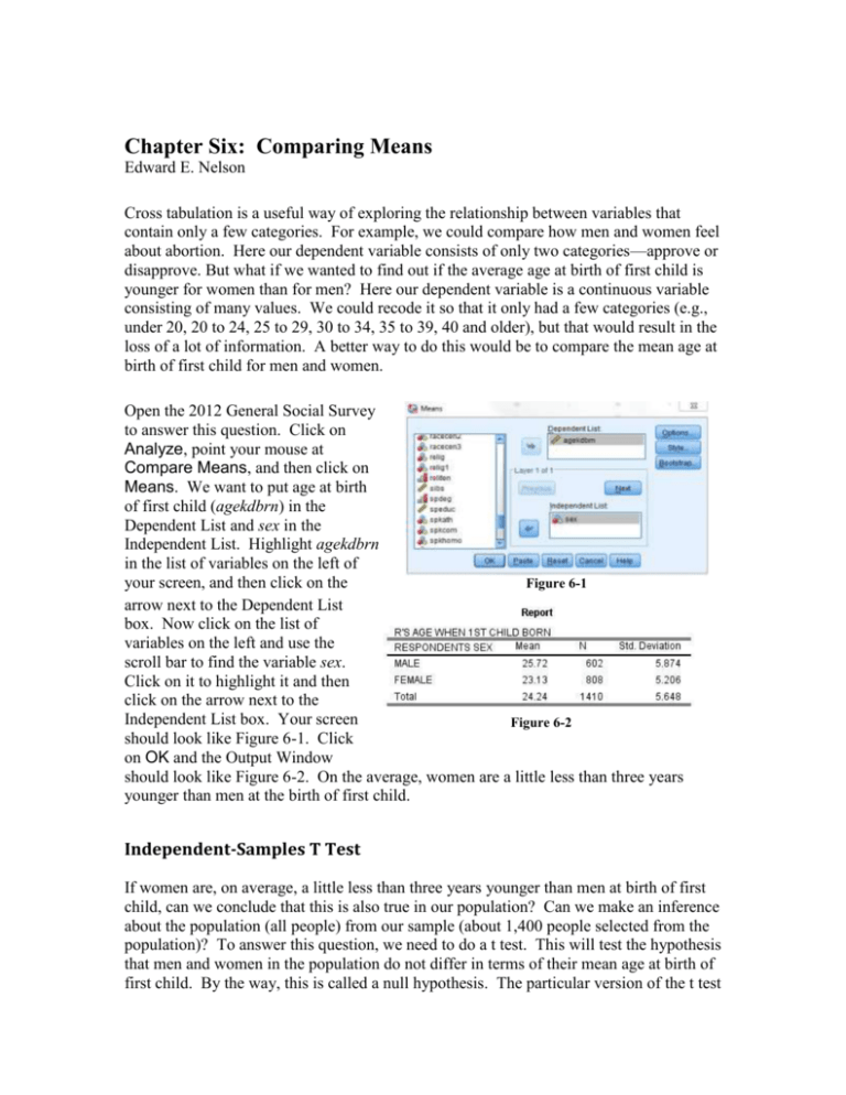
Chapter Six: Comparing Means
Edward E. Nelson
Cross tabulation is a useful way of exploring the relationship between variables that
contain only a few categories. For example, we could compare how men and women feel
about abortion. Here our dependent variable consists of only two categories—approve or
disapprove. But what if we wanted to find out if the average age at birth of first child is
younger for women than for men? Here our dependent variable is a continuous variable
consisting of many values. We could recode it so that it only had a few categories (e.g.,
under 20, 20 to 24, 25 to 29, 30 to 34, 35 to 39, 40 and older), but that would result in the
loss of a lot of information. A better way to do this would be to compare the mean age at
birth of first child for men and women.
Open the 2012 General Social Survey
to answer this question. Click on
Analyze, point your mouse at
Compare Means, and then click on
Means. We want to put age at birth
of first child (agekdbrn) in the
Dependent List and sex in the
Independent List. Highlight agekdbrn
in the list of variables on the left of
your screen, and then click on the
Figure 6-1
arrow next to the Dependent List
box. Now click on the list of
variables on the left and use the
scroll bar to find the variable sex.
Click on it to highlight it and then
click on the arrow next to the
Independent List box. Your screen
Figure 6-2
should look like Figure 6-1. Click
on OK and the Output Window
should look like Figure 6-2. On the average, women are a little less than three years
younger than men at the birth of first child.
Independent-Samples T Test
If women are, on average, a little less than three years younger than men at birth of first
child, can we conclude that this is also true in our population? Can we make an inference
about the population (all people) from our sample (about 1,400 people selected from the
population)? To answer this question, we need to do a t test. This will test the hypothesis
that men and women in the population do not differ in terms of their mean age at birth of
first child. By the way, this is called a null hypothesis. The particular version of the t test
that we will be using is called the independent-samples t test since our two samples are
completely independent of each other. In other words, the selection of cases in one of the
samples does not influence the selection of cases in the other sample. We’ll look later at
a situation where this is not true.
We want to compare our sample of men with our sample of women and then use this
information to make an inference about the population. Click on Analyze, then point
your mouse at Compare Means and then click on Independent-Samples T Test.
Find agekdbrn in the list of variables on the left and click on it to highlight it, then click
on the arrow to the left of the Test Variable box. This is the variable we want to test so it
will go in the Test Variable box.
Now click on the list of variables
on the left and use the scroll bar to
find the variable sex. Click on it to
highlight it and then click on the
arrow to the left of the Grouping
Variable box. Sex defines the two
groups we want to compare so it
will go in the Grouping Variable
box. Your screen should look like
Figure 6-3. Now we want to
Figure 6-3
define the groups so click on the
Define Groups button. This will open the Define Groups box. Since males are coded 1
and females 2, type 1 in the Group 1 box and 2 in the Group 2 box. (You will have to
click in each box before typing the value.) This tells IBM SPSS what the two groups are
that we want to compare. (If you don’t know how males and females are coded, click on
Utilities in the menu bar, then on Variables and scroll down until you find the variable
sex and click on it. The box to the right will tell you the values for males and females.
Be sure to close this box.)
Now click on Continue
and on OK in the
Independent-Samples T
Test box. Your screen
should look like Figure 64.
Figure 6-4
This table shows you the
mean age at birth of first
child for men (25.72) and
women (23.13), which is a mean difference of 2.59. It also shows you the results of two t
tests. Remember that this tests the null hypothesis that men and women have the same
mean age at birth of first child in the population. There are two versions of this test. One
assumes that the populations of men and women have equal variances (for agekdbrn),
while the other doesn’t make any assumption about the variances of the populations. The
table also gives you the values for the degrees of freedom and the observed significance
level. The significance value is .000 for both versions of the t test. Actually, this means
less than .0005 since IBM SPSS rounds to the nearest third decimal place. This
significance value is the probability that the t value would be this big or bigger simply by
chance if the null hypothesis was true. Since this probability is so small (less than five in
10,000), we will reject the null hypothesis and conclude that there probably is a
difference between men and women in terms of average age at birth of first child in the
population. Notice that this is a two-tailed significance value. If you wanted the onetailed significance value, just divide the two-tailed value in half.
Let’s work another example. This time we will compare males and females in terms of
average years of school completed (educ). Click on Analyze, point your mouse at
Compare Means, and click on Independent-Samples T Test. Click on Reset to get
rid of the information you entered previously. Move educ into the Test Variable box and
sex into the Grouping Variable box. Click on Define Groups and define males and
females as you did before. Click on Continue and then on OK to get the output window.
Your screen should look like Figures 6-5. There isn't much of a difference between men
and women in terms of years of
school completed. This time
we do not reject the null
hypothesis since the observed
significance level is greater
than .05.
Paired-Samples T Test
Figure 6-5
We said we would look at an example where the samples are not independent. (IBM
SPSS calls these paired samples. Sometimes they are called matched samples.) Let’s say
we wanted to compare the educational level of the respondent’s father and mother.
Paeduc is the years of school completed by the father and maeduc is years of school for
the mother. Clearly our samples of fathers and mothers are not independent of each
other. If the respondent’s father is in one sample, then his or her mother will be in the
other sample. One sample determines the other sample. Another example of paired
samples is before and after measurements. We might have a person’s weight before they
started to exercise and their weight after exercising for two months. Since both measures
are for the same person, we clearly do not have independent samples. This requires a
different type of t test for paired samples.
Click on Analyze, then point your mouse at Compare Means, and then click on
Paired-Samples T Test. Scroll down to maeduc in the list of variables on the left and
click on it and click on the arrow to the left of the paired Variables box to move it to
variable 1 in the paired Variables box. Now click on paeduc in the list of variables on
the left and click on it and click on the arrow to the left of the paired Variables box to
move it to variable 2 in the paired Variables box.
Your screen should look like Figure 6-6. Click on OK and your screen should look like
Figure 6-7. This table shows the mean years of school completed by mothers (11.88) and
by fathers (11.85), as well as the
standard deviations. The t-value for
the paired-samples t test is 0.351 and
the 2-tailed significance value is
0.726. (You may have to scroll
down to see these values.) This is
the probability of getting a t-value
this large or larger just by chance if
the null hypothesis is true. Since this
probability is greater than .05, we do
Figure 6-6
not reject the null hypothesis.
There is no statistical basis for
saying that the respondent’s
fathers and mothers have
different educational levels.
Notice that if we were using a
one-tailed test, then we would
divide the two-tailed significance
value of .726 by 2 which would
Figure 6-7
be .363. For a one-tailed test, we
would also not reject the null hypothesis since the one-tailed significance value is greater
than .05.
One-Way Analysis of Variance
In this chapter we have compared two groups (males and females). What if we wanted to
compare more than two groups? For example, we might want to see if age at birth of first
child (agekebrn) varies by educational level. This time let’s use the respondent’s highest
degree (degree) as our measure of
education. To do this we will use OneWay Analysis of Variance (often
abbreviated ANOVA). Click on
Analyze, then point your mouse at
Compare Means, and then click on
Means. Click on Reset to get rid of
what is already in the box. Click on
agekdbrn to highlight it and then move it
to the Dependent List box by clicking on
Figure 6-8
the arrow to the left of the box. Then
scroll down the list of variables on the left and find degree. Click on it to highlight it and
move it to the Independent List box by clicking on the arrow to the left of this box. Your
screen should look like Figure 6-8. Click on the Options button and this will open the
Means: Options box. Click in the box labeled Anova table and eta. This should put a
check mark in this box indicating that you want IBM SPSS to do a One-Way Analysis of
Variance. Your screen should look like Figure 6-9. Click on Continue and then on OK
in the Means box and your screen should look like Figure 6-10.
In this example, the independent
variable has five categories: less than
high school, high school, junior
college, bachelor, and graduate.
Figure 6-10 shows the mean age at
birth of first child for each of these
groups and their standard deviations,
as well as the Analysis of Variance
table including the sum of squares,
degrees of freedom, mean squares, the
F-value and the observed significance
value. (You will have to scroll down
to see the Analysis of Variance table.)
The significance value for this
example is the probability of getting a
F-value of 76.279 or higher if the null
hypothesis is true. Here the null
Figure 6-9
hypothesis is that the mean age at birth
of first child is the same for
all five-population groups.
In other words, that the mean
age at birth of first child for
all people with less than a
high school degree is equal to
the mean age for all with a
high school degree and all
those with a junior college
degree and all those with a
bachelor’s degree and all
those with a graduate degree.
Since this probability is so
Figure 6-10
low (<.0005 or less than 5
out of 10,000), we would
reject the null hypothesis and conclude that these population means are probably not all
the same.
There is another procedure in IBM SPSS that does One-Way Analysis of Variance and
this is called One-Way ANOVA. This procedure allows you to use several multiple
comparison procedures that can be used to determine which groups have means that are
significantly different.
Conclusion
This chapter has explored ways to compare the means of two or more groups and
statistical tests to determine if these means differ significantly. These procedures would
be useful if your dependent variable was continuous and your independent variable
contained a few categories. The next chapter looks at ways to explore the relationship
between pairs of variables that are both continuous.
Chapter Six Exercises
Use the GSS12A data set for all these exercises.
1. Compute the mean age (age) of respondents who voted for Obama or McCain
(pres08). Which group had the youngest mean age and which had the oldest mean
age?
2. Use the independent-samples t test to compare the mean family income (income06) of
men and women (sex). Which group had the highest mean income? Was the
difference statistically significant (i.e., was the significance value less than .05)?
3. Use the independent-samples t test to compare the mean age (age) of respondents
who believe and do not believe in life after death (postlife). Which group had the
highest mean age? Was the difference statistically significant (i.e., was the
significance value less than .05)?
4. Use One-Way Analysis of Variance to compare the mean years of school completed
(educ) for respondents who voted for Obama or McCain (pres08). Which group had
the most education and which had the least education? Was the F-value statistically
significant (i.e., was the significance value less than .05)?