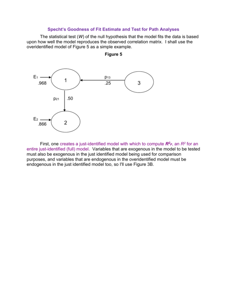
Specht’s Goodness of Fit Estimate and Test for Path Analyses
The statistical test (W) of the null hypothesis that the model fits the data is based
upon how well the model reproduces the observed correlation matrix. I shall use the
overidentified model of Figure 5 as a simple example.
Figure 5
E1
.968
1
p21
E2
.866
p13
.25
3
.50
2
First, one creates a just-identified model with which to compute R2F, an R2 for an
entire just-identified (full) model. Variables that are exogenous in the model to be tested
must also be exogenous in the just identified model being used for comparison
purposes, and variables that are endogenous in the overidentified model must be
endogenous in the just identified model too, so I'll use Figure 3B.
To obtain R2F one simply obtains the product of the squares of all the error paths
and subtracts from one. For Figure 3B,
R2F = 1 - (.968)2(.775)2 = .437.
Next, one computes R2R , an R2 for the overidentified (reduced) model being
tested. Again, one simply obtains the product of the squared error path coefficients and
subtracts from one. For Figure 5, R2R = 1 - (.968)2(.866)2 = .297. The smaller R2R is
relative to R2F , the poorer the fit, and the fit here looks poor indeed. Were the
overidentified model to perfectly reproduce the original correlation matrix, R2R would
equal R2F, and the fit would be perfect.
We next compute Q, a measure of the goodness of fit of our overidentified
1  RF2
Q

model, relative to a perfectly fitting (just identified) model.
. For our
1  RR2
example, Q = (1 -.437)/(1 -.297) = .801. A perfect fit would give a Q of one; less than
perfect fits yield Q's less than one. Q can also be computed simply by computing the
product of the squares of the error path coefficients for the full model and dividing by the
square of the products of the error path coefficients for the reduced model. For our
(.968) 2 (.775) 2
model, Q 
 .801 .
(.968) 2 (.866) 2
Finally, we compute the test statistic, W = -(N - d)  ln(Q) where N = sample
size (let us assume N = 100), d = number of overidentifying restrictions (number of
paths eliminated from the full model to yield the reduced model), and ln = natural
logarithm. For our data, W = -(100 - 1) * ln(.801) = 21.97. W is evaluated with the
chi-square distribution on d degrees of freedom. For our W, p <.0001 and we conclude
that the model does not fit the data well. If you compute W for Figure 4A or 4B you will
obtain W = 0, p = 1.000, indicating perfect fit for those models.
The overidentified model (Figure 5) we tested had only one restriction (no p23), so
we could have more easily tested it by testing the significance of p23 in Figure 3B. Our
overidentified models may, however, have several such restrictions, and the method I
just presented allows us simultaneously to test all those restrictions. Consider the
overidentified model in Figure 6.
Figure 6
SES
1
E3
p31
.410
r12 .3
.912
p43
nACH
3
.420
p42
.503
IQ
2
GPA
4
.710
E4
The just identified model in Figure 1 is an appropriate model for computing R2F.
Figure 1
SES
1
p41 = .009
p31 = .398
nACH
3
r12 = .3
p43 = .416
GPA
4
p32 = .041
E3
p42 = .501
E4
IQ
2
In the just-identified model E3  1  R32.12  .911 and E 4  1  R42.123  .710 . For
our overidentified model E3  1  R32.1  .912 and E4  1  R42.23  .710 .
R2F = 1 - (.911)2(.710)2 = .582. R2R = 1 - (.912)2(.710)2 = .581. Q = (1 - .582)/(1 - .581)
= .998. If N = 100, W = -(100 - 2) * ln(.998) = 0.196 on 2 df (we eliminated two paths), p
= .91, our overidentified model fits the data well.
Let us now evaluate three different overidentified models, all based on the same
correlation matrix. Variable V is a measure of the civil rights attitudes of the Voters in
116 congressional districts (N = 116). Variable C is the civil rights attitude of the
Congressman in each district. Variable P is a measure of the congressmen's
Perceptions of their constituents' attitudes towards civil rights. Variable R is a measure
of the congressmen's Roll Call behavior on civil rights. Suppose that three different a
priori models have been identified (each based on a different theory), as shown in
Figure 8.
Figure 8
Just-Identified Model
C
.867
EC
.498
.324
.075
V
R
.560
.366
.507
.556
ER
P
.595
EP

For the just-identified model, R2F = 1 - (.867)2(.595)2(.507)2 = .9316.
Model X
C
.766
EC
.643
.327
V
R
.613
.510
.738
ER
P
.675
EP

For Model X, R2R = 1 - (.766)2(.675)2(.510)2 = .9305.
Model Y
C
.867
EC
.498
.327
V
R
.613
.643
.510
ER
P
.766
EP

For Model Y, R2R = 1 - (.867)2(.766)2(.510)2 = .8853.
Model Z
C
.867
EC
.498
.327
V
R
.613
.366
.510
.556
ER
P
.595
EP

For Model Z, R2R = 1 -(.867)2(.595)2(.510)2 = .9308.

Goodness of fit Qx = (1 - .9316)/(1 - .9305) = .0684/.0695 = .9842.

Qy = .0684/(1 - .8853) = .5963.

Qz = .0684/(1 - .9308) = .9884.

It appears that Models X and Z fit the data better than does Model Y.
Wx = -(116 - 2)  ln(.9842) = 1.816. On 2 df (two restrictions, no paths from V to
C or to R), p = .41. We do not reject the null hypothesis that Model X fits the data.
WY = -(116 - 2)  ln(.5963) = 58.939, on 2 df, p <.0001. We do reject the null and
conclude that Model Y does not fit the data.
WZ = -(116 - 1)  ln(.9884) = 1.342, on 1 df (only one restriction, no V to R direct
path) p = .25. We do not reject the null hypothesis that Model Z fits the data. It seems
that Model Y needs some revision, but Models X and Z have passed this test.
Sometimes one can test the null hypothesis that one reduced model fits the data
as well as does another reduced model. One of the models must be nested within the
other -- that is, it can be obtained by eliminating one or more of the paths in the other.
For example, Model Y is exactly like Model Z except that the path from V to P has been
eliminated in Model Y. Thus, Y is nested within Z. To test the null, we compute
W = -(N -d)  ln[(1 - M1)/(1 - M2)] . M2 is for the model that is nested within the other,
and d is the number of paths eliminated from the other model to obtain the nested
model. For Z versus Y, on d = 1 df, W = -(116 - 1) * ln[(1 - .9308)/(1 - .8853) = 58.112, p
< .0001. We reject the null hypothesis. Removing the path from V to P significantly
reduced the fit between the model and the data.
Karl L. Wuensch
Department of Psychology
East Carolina University
Greenville, NC 27858