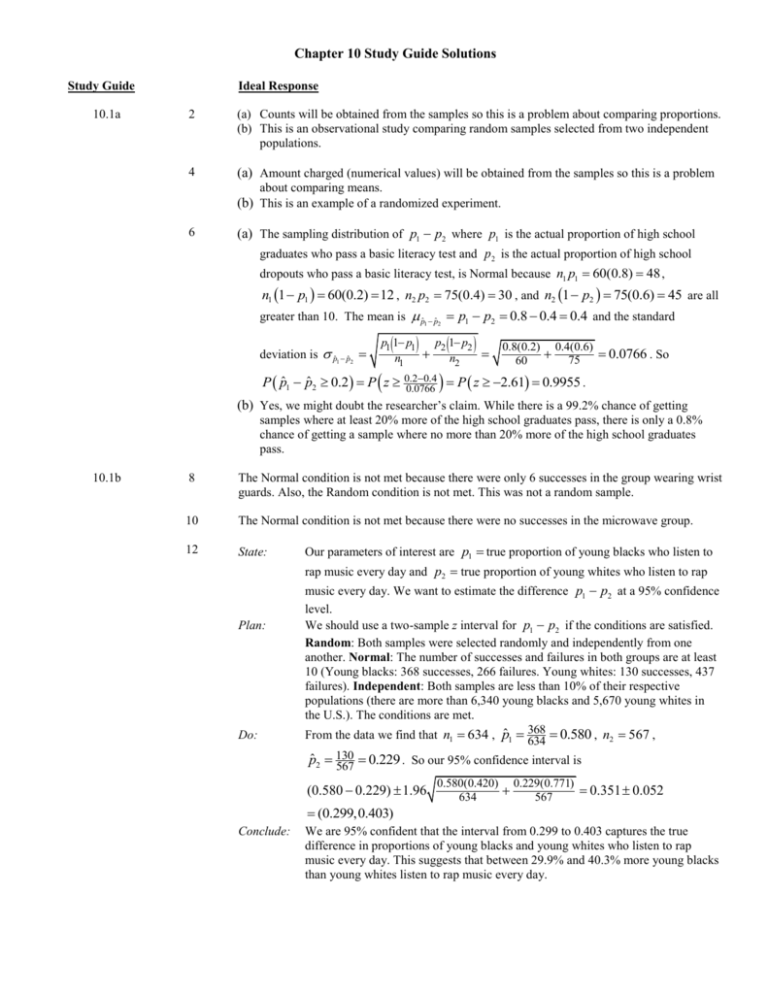
Chapter 10 Study Guide Solutions
Study Guide
10.1a
Ideal Response
2
(a) Counts will be obtained from the samples so this is a problem about comparing proportions.
(b) This is an observational study comparing random samples selected from two independent
populations.
4
(a) Amount charged (numerical values) will be obtained from the samples so this is a problem
about comparing means.
(b) This is an example of a randomized experiment.
6
(a) The sampling distribution of p1  p2 where p1 is the actual proportion of high school
graduates who pass a basic literacy test and p 2 is the actual proportion of high school
dropouts who pass a basic literacy test, is Normal because n1 p1  60(0.8)  48 ,
n1 1  p1   60(0.2)  12 , n2 p2  75(0.4)  30 , and n2 1  p2   75(0.6)  45 are all
greater than 10. The mean is  pˆ1  pˆ 2  p1  p2  0.8  0.4  0.4 and the standard
deviation is  pˆ1  pˆ 2 




p1 1 p1
p2 1 p2
 n

n1
2
0.8(0.2) 0.4(0.6)
 75  0.0766 . So
60
0.4
P  pˆ1  pˆ 2  0.2   P  z  0.2
0.0766   P  z  2.61  0.9955 .
(b) Yes, we might doubt the researcher’s claim. While there is a 99.2% chance of getting
samples where at least 20% more of the high school graduates pass, there is only a 0.8%
chance of getting a sample where no more than 20% more of the high school graduates
pass.
10.1b
8
The Normal condition is not met because there were only 6 successes in the group wearing wrist
guards. Also, the Random condition is not met. This was not a random sample.
10
The Normal condition is not met because there were no successes in the microwave group.
12
State:
Our parameters of interest are p1  true proportion of young blacks who listen to
rap music every day and p2  true proportion of young whites who listen to rap
Plan:
Do:
music every day. We want to estimate the difference p1  p2 at a 95% confidence
level.
We should use a two-sample z interval for p1  p2 if the conditions are satisfied.
Random: Both samples were selected randomly and independently from one
another. Normal: The number of successes and failures in both groups are at least
10 (Young blacks: 368 successes, 266 failures. Young whites: 130 successes, 437
failures). Independent: Both samples are less than 10% of their respective
populations (there are more than 6,340 young blacks and 5,670 young whites in
the U.S.). The conditions are met.
 0.580 , n2  567 ,
From the data we find that n1  634 , pˆ1  368
634
pˆ 2  130
 0.229 . So our 95% confidence interval is
567
0.580(0.420) 0.229(0.771)
(0.580  0.229)  1.96

 0.351  0.052
634
567
 (0.299,0.403)
Conclude:
We are 95% confident that the interval from 0.299 to 0.403 captures the true
difference in proportions of young blacks and young whites who listen to rap
music every day. This suggests that between 29.9% and 40.3% more young blacks
than young whites listen to rap music every day.
Chapter 10 Study Guide Solutions
14
(a) State:
Our parameters of interest are p1  true proportion of older black men who fear
crime and p2  true proportion of older black women who fear crime. We want to
estimate the difference p1  p2 at a 90% confidence level.
Plan:
Do:
We should use a two-sample z interval for p1  p2 if the conditions are satisfied.
Random: Both samples were selected randomly and independent from one
another. Normal: The number of successes and failures in both groups are at least
10 (Older black men: 46 successes, 17 failures. Older black women: 27 successes,
29 failures). Independent: Both samples are less than 10% of their respective
populations (there are more than 630 older black men and 560 older black women
in Atlantic City, NJ). The conditions are met.
From the data we find that n1  63 , pˆ1  46  0.73 , n2  56 , pˆ 2  27  0.482
63
56
So our 90% confidence interval is
0.73(0.27) 0.482(0.519)
(0.730  0.482)  1.645

 0.248  0.143
63
56
 (0.105,0.391)
Conclude:
We are 90% confident that the interval between 0.105 and 0.391 captures the true
difference in the proportions of older black men and older black women who fear
crime. This interval suggests that between 10.5% and 39.1% more older black men
than older black women fear crime.
(b) Since the interval does not contain 0, there is convincing evidence that the two proportions
are not the same.
10.1c
16
H o : p1  p2  0 versus Ha : p1  p2  0 where p1 is the actual proportion of high school
freshman in Illinois who use anabolic steroids and p 2 is the actual proportion of high school
seniors in Illinois who use anabolic steroids.
18
(a) State:
Plan:
Do:
We want to perform a test at the   0.5 significance level of the hypotheses
stated in Exercise 16.
We should use a two-sample z test for p1  p2 if the conditions are satisfied.
Random: Both samples were selected randomly and independent from one
another. Normal: The number of successes and failures in both groups are at least
10 (Freshmen: 34 successes, 1645 failures. Seniors: 24 successes, 1342 failures).
Independent: Both samples are less than 10% of their respective populations
(there are more than 16,790 freshmen and 13,660 seniors in Illinois). The
conditions are met.
The proportions of those using anabolic steroids in each group are
34  0.0203 , p
24  0.0176 . The pooled proportion is
ˆ 2  1366
pˆ1  1679
3424  58  0.0190 . The test statistic is
pˆ C  1679
1366 3045
z
(0.02030.0176)0
(0.019)(0.981)  (0.019)(0.981)
1679
1366
 0.54 .
Since this is a two-sided test the P-value is 2P( z  0.54)  2(0.2946)  0.5892
Conclude:
(b) State:
Plan:
Do:
Since the P-value is greater than 0.05, we fail to reject the null hypothesis. We do
not have enough evidence to conclude that there is a difference in the actual
proportions of freshmen and seniors in Illinois who use anabolic steroids.
We want to estimate the difference p1  p2 at a 95% confidence level.
We should use a two-sample z interval for p1  p2 if the conditions are satisfied.
We checked the conditions in part (a) and they have been met.
From the data we find that n1  1679 , pˆ1  0.0203 , n2  1366 , pˆ 2  0.0176
So our 95% confidence interval is
0.0203(0.9797) 0.0176(0.9824)
(0.203  0.0176)  1.96

 0.0027  0.0097
1679
1366
 (0.007,0.0124)
Chapter 10 Study Guide Solutions
22
Conclude:
We are 95% confident that the interval from –0.007 to 0.0124 captures the true
difference in the proportions of freshmen and seniors who use anabolic steroids.
This is consistent with our answer to part (a). In both cases we decided that 0 was
a plausible value for the difference in the proportions.
(a) State:
We want to perform a test at the   0.5 significance level of the hypotheses
H o : p1  p2  0 versus Ha : p1  p2  0 where p1 is the actual proportion of
patients like the ones in the study who would have a stroke when taking aspirin
alone and p 2 is the actual proportion of patients like the ones in the study who
would have had a stroke when taking both drugs.
We should use a two-sample z test for p1  p2 if the conditions are satisfied.
Random: This was a randomized comparative experiment. Normal: The number
of successes and failures in both groups are at least 10 (Aspirin alone: 206
successes, 1443 failures. Additional medicine group: 157 successes, 1493 failures).
Independent: Due to the random assignment, these two groups of patients can be
viewed as independent. Individual observations in each group should also be
independent: knowing whether one patient had a stroke or not gives no
information about another patient. The conditions are met.
206  0.125 ,
The proportions of stroke victims in each group are pˆ1  1649
157  0.095 . The pooled proportion is p
206157  363  0.11 .
ˆ C  1649
pˆ 2  1650
1650 3299
Plan:
Do:
The test statistic is z 
(0.1250.095)0
(0.11)(0.89)  (0.11)(0.89)
1649
1650
 2.75 .
Since this is a two-sided test the P-value is 2P( z  2.75)  2(0.003)  0.006
Conclude: Since the P-value is less than 0.05, we reject the null hypothesis. We have enough
evidence to conclude that there is a difference in the proportions of patients like
the ones in this study who suffer strokes depending on whether they take aspirin
alone or take the additional medication as well.
(b) A Type I error would be to conclude that there is a difference between the stroke rates for
the two treatments when there is no difference and a Type II error would be to conclude
that there is no difference between the stroke rates of people on the two different treatments
when there actually is. A Type II error would be more serious in this case because we
would not market a drug that would reduce the number of strokes that people suffer.
24
10.1 MC
(a) We should use a two-sample z test for p1  p2 if the conditions are satisfied. Random: This
was a randomized comparative experiment. Normal: The number of successes and failures
in both groups are at least 10 (Acupuncture group: 34 successes, 46 failures. Control group:
21 successes, 59 failures). Independent: Due to the random assignment, these two groups of
women can be viewed as independent. Individual observations in each group should also be
independent: knowing whether one woman became pregnant gives no information about
another woman. The conditions are met.
(b) If there is no difference in pregnancy rates of women who receive acupuncture and those
who don’t, there is a 1.52% chance of seeing as many more pregnancies while receiving
acupuncture as we did.
(c) Since the P-value was less than 0.05, we reject the null hypothesis. We have enough
evidence to conclude that the proportion of pregnancies among women like these who
receive acupuncture is higher than for those who do not.
(d) This study was not blind. The women who received acupuncture knew that they had
received the treatment and those in the control group knew that they had not received the
treatment. This may affect their behavior (even unconsciously) in such a way as to affect
whether they became pregnant or not.
29. B
30. D
31. B
32. E
Chapter 10 Study Guide Solutions
10.2a
36
(a) The sampling distribution of M  W where p1 is approximately normal with mean
 M W   M  W  69.3  64.5  4.8 inches and the standard deviation is
 M W   M2   W2  (2.8)2  (2.5)2  3.75 .


4.8  P z  0.75  0.7734 .
(b) P  M  W  2   P z  23.75


38
(a) The distribution of xM  xW is approximately normal with mean
 M W   M  W  69.3  64.5  4.8 inches and standard deviation
x
M
 xW

2
M
nM

W2
nW


(2.8)2
16

(2.5)2
9
 1.09 inches.

4.8  P z  2.57  0.9949
(b) P  xM  xW  2   P z  21.09


(c) No. It is almost certain (a 99.49% chance) that the sample mean height for young women is
more than 2 inches less than the sample mean height for the young men.
10.2b
58
(a) If people were allowed to choose which group they wanted to be in, it is likely that all those
who choose one particular treatment (sleep deprivation, for example) might be
systematically different from those who choose to be in the other treatment group.
(b) Based on the dotplot from Fathom, a difference of 15.92 between the means is quite rare.
Only about 5 out of the 1000 differences were that big. We would conclude that the mean
increase in score is significantly higher for those who were allowed to sleep than for those
who were sleep deprived.
(c) Since we rejected the null hypothesis (of no difference), this could have been a Type I error
– rejecting the null hypothesis when it is really true.
39
No. The Normal condition is not met with this data set. There are fewer than 30 observations in
each group and the stemplot for Males shows skewness.
40
Yes. The conditions are met. Even though there is an outlier in the South African distribution,
the two sample sizes are large enough to make the two-sample t procedures fairly accurate.
41
No. The Independent condition is not met in this data set. We have data from more than 10% of
Islamic nations.
42
No. The Random condition was not met in this study. The words chosen from each article were
the first words (either 100 or 200) in the article. It may be that the word length differs in different
locations in the articles.
44
(a) The centers of the two groups seem to be quite different, with red flowers being longer. The
red flowers also seem to have more variability to their lengths.
(b) State:
Our parameters of interest are 1  the actual mean length of red flowers and
Plan:
 2  the actual mean length of yellow flowers. We want to estimate the
difference 1  2 at a 95% confidence level.
We should use a two-sample t interval for 1  2 if the conditions are satisfied.
Do:
Random: Both samples were randomly selected independently of one another.
Normal: Both sample sizes were less than 30. However, the dotplots given in the
problem do not indicate serious skewness or large outliers. Independent: Both
samples are less than 10% of their respective populations (there are more than
230 red flowers and 150 yellow flowers). The conditions are met.
From the data we find that n1  23 , x1  39.698 , s1  1.786 , n2  15 ,
x2  36.18 , and s2  0.975 . We will use the conservative degrees of freedom
which is 14 in this case. So our 95% confidence interval is
(36.698  36.18)  2.145
(1.786)2 (0.975)2
 15  3.518  0.964  (2.554, 4.482)
23
Chapter 10 Study Guide Solutions
Conclude:
We are 95% confident that the interval from 2.554 to 4.482 captures the
difference in actual mean length of red flowers and yellow flowers. This suggests
that the mean length of red flowers is between 2.554 mm and 4.482 mm larger
than the mean length of the yellow flowers.
(c) Since 0 is not in this interval, it does support the researchers’ belief that the two varieties
have different lengths
46
(a) The use of the two-sample t procedure is still justified because the t procedures are robust
against non-Normality in the populations with such large samples.
(b) State:
Our parameters of interest are 1  the actual mean reliability rating of Anglo
customers and  2  the actual mean reliability rating of Hispanic customers. We
want to estimate the difference 1  2 at a 95% confidence level.
Plan:
Do:
We should use a two-sample t interval for 1  2 if the conditions are satisfied.
Random: Both samples were randomly selected independently of one another.
Normal: Both sample sizes were at least 30. Independent: Both samples are less
than 10% of their respective populations ((there are likely more than 920 Anglo
customers of the bank and 860 Hispanic customers of the bank). The conditions
are met.
From the data we find that n1  92 , x1  6.37 , s1  0.60 , n2  86 , x2  5.91 ,
and s2  0.93 . We will use the conservative degrees of freedom which is 85 in
this case. So our 95% confidence interval is
(0.60)2 (0.93)2
(6.37  5.91)  1.988
 86  0.46  0.235  (0.225,0.695)
92
Conclude:
We are 95% confident that the interval from 0.225 to 0.695 captures the actual
difference in mean reliability rating for Anglos and Hispanics. This suggests that
the mean reliability rating for Anglos is between 0.225 and 0.695 higher than the
mean reliability rating for Hispanics.
(c) If we repeatedly took random samples of 92 Anglos and 86 Hispanics and each time
constructed a 95% confidence interval in this same way, about 95% of the resulting intervals
would capture the actual difference in mean reliability rating.
10.2c
52
(a) Breast-feeding mothers have a lower mean mineral content  x1  3.587, s1  2.506  with
more variability than other mothers  x2  0.309, s2  1.298 . Both distributions appear
slightly right-skewed.
(b) State:
We want to perform a test at the   0.05 significance level of
H o : 1   2  0 versus H a : 1  2  0 where 1  the actual mean percent
Plan:
Do:
change in mineral content for breastfeeding women and  2  the actual mean
percent change in mineral content for women who were neither pregnant nor
lactating.
We should use a two-sample t test if the conditions are satisfied. Random: Both
samples were selected randomly independently of one another. Normal: Since
the number of observations in the control group is less than 30 we check the
boxplots. Independent: Both samples are less than 10% of their respective
populations (there are more than 470 breastfeeding women and 220 non-pregnant
and non-lactating women). The conditions are met.
From the data we find that n1  47 , x1  3.587 , s1  2.506 , n2  22 ,
x2  0.309 , and s2  1.298 . We will use the conservative degrees of freedom
which is 21 in this case. The test statistic is t 
Conclude:
( 3.5870.309)0
(0.60)2 (0.93)2
 86
92
 8.498 . This
is a one-sided test, so the P-value is P(t  8.498)  0
Since the P-value is less than 0.05, we reject the null hypothesis. We have
enough evidence to conclude that breastfeeding women have a larger mean
percent bone mineral loss than women who are neither pregnant nor lactating.
(c) Since this was not a randomized controlled experiment we cannot conclude that
Chapter 10 Study Guide Solutions
breastfeeding causes bone mineral loss.
(d) State:
We want to estimate the difference 1  2 at a 95% confidence level.
Plan:
Do:
We should use a two-sample t interval for 1  2 if the conditions are satisfied.
We checked the conditions in part (b) and they were met.
Using 21 df, our 95% confidence interval is
(2.506)2 (1.298)2
(3.587  0.309)  2.080
 22  3.896  0.954
47
 (4.85, 2.942)
Conclude:
53
(a) State:
Plan:
Do:
We are 95% confident that the interval from -4.85 to -2.942 captures the difference
in actual mean percent of bone mineral loss in breastfeeding women and nonpregnant and non-lactating women. This interval suggests that the mean percent of
bone3 mineral loss in breastfeeding women is between 4.85% and 2.942% more than
for women who are neither pregnant nor lactating. This interval not only addresses
the plausibility of the two means being the same, but also gives a range of plausible
values for the difference in the two means.
We want to perform a test at the   0.05 significance level of H o : 1   2  0
versus H a : 1  2  0 where 1  the actual mean number of words spoken per
day by female students and  2  the actual mean number of words spoken by
male students.
We should use a two-sample t testif the conditions are satisfied. Random: Both
samples were selected randomly. Normal: Both samples had more than 30
observations. Independent: Both samples are less than 10% of their respective
populations (there are more than 560 female students at a large university and 560
male students at a large university). The conditions are met.
From the data we find that n1  56 , x1  16,177 , s1  7520 , n2  56 , x2  16,569 ,
and s2  9108 . We will use the conservative degrees of freedom which is 55 in this
case. The test statistic is t 
(1617716569)0
(7520)2 (9108)2
 56
56
 0.248 . This is a two-sided test, so the
P-value is 2P(t  0.248)  2(0.4025)  08050
Conclude: Since the P-value is greater than 0.05, we fail to reject the null hypothesis. We do
not have enough evidence to conclude that male students and female students speak
a different number of words per day on average.
(b) If males and females speak the same number of words per day on average, then we have
about an 80% chance of selecting a sample where the difference between the average
number of words spoken per day by males and females is as large as or larger than the
difference we actually saw.
10.2 MC
59
(a) Two-sample t test. Each car has a different brand of tire on it. There is no obvious way to
pair one observation of a Brand A tire with one observation of a Brand B tire.
(b) Paired t test. The subjects are each subjected to both treatments. So we would take the
differences in productivity for each subject from when they listened to music and when they
didn’t.
(c) Two-sample t test. Each person was only given one treatment. Then the two groups were
compared.
60
(a) Paired t test. Pairs of pigs who were littermates were used, with one in each pair getting one
treatment and the other pig in the pair getting the other treatment.
(b) Two-sample t test. There is no connection between the male and female professors. They are
not paired in any way.
(c) Two-sample t test. The treatments were randomly assigned to the plots. There is no way to
pair a plot with one treatment with a plot with the other treatment.
67. D
68. A
69. A
70. B